Summary Lab #11
Lab #11 incorporates the Bayes Filter tested and simulated from the previous lab into a real-world example, integrating the real-world sensing developed on the Artemis Nano board for visualization and localization. With this dynamic sensing script, the Bayes Filter is applicable to the specific environment created in the Tang electronics lab and the robots on-board sensing is available for usage in improving the determination method for the stunt car’s specific location. With this method integrated, the stunt car is able to determine relative position with high accuracy that is perfect for dynamic, position-based motion in space (similar to the simulation in lab 10).
Lab #11 Outcomes
Lab 11 Simulator Final Plot
Major time was lost while troubleshooting backend issues with the simulator for my 2023 MacBook Pro (Apple M2 Pro Chip, 16 GB) in case this is helpful for future reference. After successfully reinstalling the Box2D wheel file and the complimentary pQt files, the following video and graph was attained from running “lab11_sim.ipynb:”
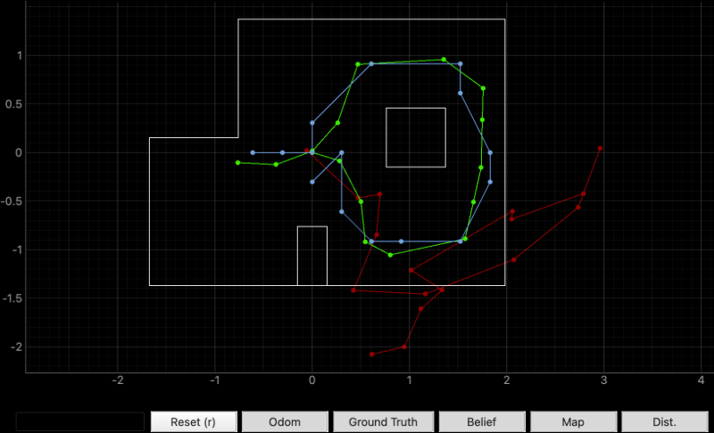
Real Life Initialization of the Environment with Bayes Filter
First, I integrated the following helper functions on both the Artemis Nano (C++) and the Jupyter Notebook UI (Python) to control rotating sensing and post-processing. First, the “SENSE_INIT” function is utilized on the stunt car in order to meet the 360 sensing requirement at every 20 degree interval:
Arduino Code (C++)
case SENSE_INIT: {
     // Sample 18 points (20 degree increments)
     yaw_calculator();
     float initial_yaw = yaw_deg;
     for(int i = 0; i < 18; i++) {
       yaw_sample_points[i] = initial_yaw + i * 20;
       // Normalize to [0, 360)
       while(yaw_sample_points[i] >= 360) {
         yaw_sample_points[i] -= 360;
       }
       while(yaw_sample_points[i] < 0) {
         yaw_sample_points[i] += 360;
       }
       Serial.print("Target ");
       Serial.print(i);
       Serial.print(": ");
       Serial.print(yaw_sample_points[i]);
       Serial.println("°");
     }
     sense_index = 0;
     ori_PID_target = yaw_sample_points[0];
     ori_integral_error = 0.0;
     ori_PID_prev_error = 0.0;
     ori_PID_last_time = millis();
     ori_PID_control = true;
     sense_activate = true;

     tx_estring_value.clear();
     tx_estring_value.append("Area Sense Initialized - Starting at ");
     tx_estring_value.append(initial_yaw);
     tx_estring_value.append("°");
     tx_characteristic_string.writeValue(tx_estring_value.c_str());
     Serial.println("Successful Area Sense Initialization");
     break;
   }
Additionally, the “perform_observation_loop” function is updated to meet the requirements of calling “SENSE_INIT” and storing the data. Complimentary to this function, “notif_callback_motion” is defined to compile the transmitted data into pre-defined arrays that are available for the Bayes post-processing:
Jupyter Notebook (Python)
    def perform_observation_loop(self, rot_vel=120):
        """
        Initiates a 360° rotation and collects 18 yaw/TOF readings from the
        real robot over BLE. Uses notification callback for real-time data.

        Args:
            rot_vel: Not used directly (gains are hardcoded on Arduino),
                     kept for interface compatibility.

        Returns:
            sensor_ranges   -- np.array (18,1) distances in meters
            sensor_bearings -- np.array (18,1) yaw angles in degrees
        """
        sensor_ranges = np.zeros((18, 1))
        sensor_bearings = np.zeros((18, 1))

        # Reset state
        self.angle_list = []
        self.distance_list = []
        self.scan_complete = False

        # Register notification handler
        self.ble.start_notify(self.ble.uuid['RX_STRING'], self.notif_callback_motion)

        # Push orientation PID gains before scanning
        print("Setting orientation PID Gains")
        self.ble.send_command(CMD.PID_ORI_GAINS, f"{3.0}|{0.15}|{0.0}")

        # Trigger the 360° area scan on the Arduino
        print("Starting area sense scan")
        self.ble.send_command(CMD.SENSE_INIT, "")

        # Stop notifications
        self.ble.stop_notify(self.ble.uuid['TX_STRING'])

        n = len(self.angle_list)
        print(f"Scan finished: {n} readings collected.")

        # Pack into output arrays
        for i in range(min(n, 18)):
            sensor_ranges[i]   = self.distance_list[i] / 1000.0
            sensor_bearings[i] = self.angle_list[i]

        self.obs_range_data = sensor_ranges
        return sensor_ranges, sensor_bearings

# ── Standalone callback (if you prefer module-level, not method) ───────────────
def notif_callback_motion(UUID, Notif_Array):
    """
    Module-level version. Requires angle_list / distance_list to be
    in the enclosing scope (e.g. notebook globals).
    """
    input_data = ble.bytearray_to_string(Notif_Array).strip()

    if "Scan Complete" in input_data:
        print("[INFO] Scan complete signal received.")
        return

    if input_data.startswith("Reading") and "Angle=" in input_data:
        try:
            after_colon = input_data.split(":", 1)[1].strip()
            parts  = after_colon.split(",")
            angle  = float(parts[0].split("=")[1].strip())
            dist   = float(parts[1].split("=")[1].strip())
            angle_list.append(angle)
            distance_list.append(dist)
            print(f"  → angle={angle:.1f}°, dist={dist:.1f}mm")
        except Exception as e:
            print(f"[WARN] Skipped malformed line: '{input_data}' | Error: {e}")
With these scripts compiled, the localization method was computed at each of the marked out locations in the map, including (5, 3), (5, -3), (0, 3), (0, 0), and (3, 2). The car was oriented facing the wall as shown in the following photo:
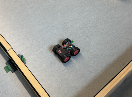
Figure 2: Orientation of the stunt car within the wood-frame environment in-lab
- Initial / Position (0, 0)
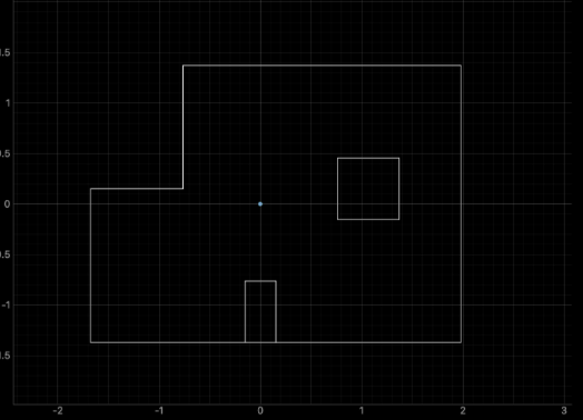
Figure 3: Localization Plotter reconstructed at Position (0, 0) (Blue) with the Real Point (Green)
Ground Truth Pose: (0.000, 0.000, 0.000) Computed Belief Pose: (0.000, 0.000, -150.0) Resultant Error: (-0.000, -0.000, -150.0)
- Position (5, 3)
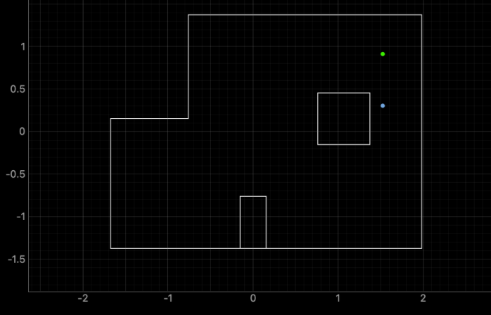
Figure 3: Localization Plotter reconstructed at Position (5, 3)(Blue) with the Real Point (Green)
Ground Truth Pose: (1.524, 0.914, 0.000) Computed Belief Pose: (1.524, 0.305, -30.0) Resultant Error: (-0.000, 0.610, -30.0)
- Position (5, -3)
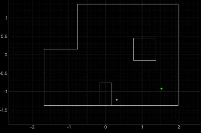
Figure 4: Localization Plotter reconstructed at Position (5, -3) (Blue) with the Real Point (Green)
Ground Truth Pose: (1.524, -0.914, 0.000) Computed Belief Pose: (0.305, -1.219, 90.0) Resultant Error: (1.219, 0.305, 90.0)
- Position (0, 3)
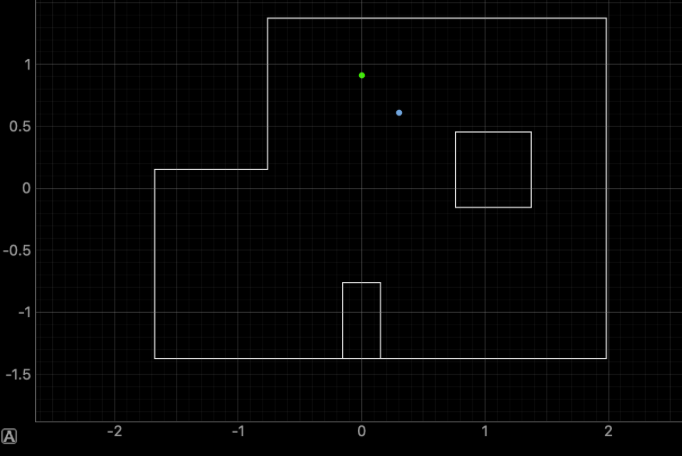
Figure 5: Localization Plotter reconstructed at Position (0, 3) (Blue) with the Real Point (Green)
Ground Truth Pose: (0.000, 0.914, 0.000) Computed Belief Pose: (0.305, 0.610, 70.0) Resultant Error: (-0.305, 0.305, 70.0)
- Position (-3, -2)
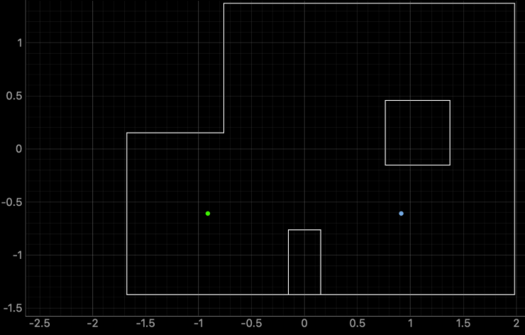
Figure 6: Localization Plotter reconstructed at Position (-3, -2) [Blue] with the Real Point [Green]
Ground Truth Pose: (-0.914, -0.610, 0.000) Computed Belief Pose: (0.914, -0.610, 90.0) Resultant Error: (-1.829, 0.000, 90.0)
Overall, the stunt car performed moderately well in certain areas of the environment with lower belief pose error, but others with significant error. At positions (5, 3) and (0, 3), the estimation method has generally accurate at providing an idea of the relative location of the stunt car, which makes sense considering the unique localization outputs at these regions. In contrast, position (5, -3) and (-3, -2) yielded significant error, likely due to measurements in large empty areas that are more susceptible to sampling errors. Although the method is more refined, the orientation sensing method discussed on the Artemis Nano Board still has some non-axial motion associated with its rotation. This would likely lead to some off values in the sensing sampling method that would lead to such significant error.
Discussion
Lab #11 was a great opportunity to implement the Bayes filter in a real-life example and work on integrating localization to the actual stunt car environment. While lab #10 provided a great simulated use cases of this example, lab #11 was a helpful next step towards testing these sensing methods through the code developed early in the semester. Although there were some errors, this is still tunable for future usage. This lab was completed with Jamison Taylor, and assisted from AI tools for minor debugging.