Summary Lab #10
Lab #10 incorporates grid-based localization with the Bayes Filter to provide estimates of robot positions in a simulated environment. More specifically, with the Bayes Filter, a distinct framework is established for estimating the stunt car’s positions over time through control inputs and observations. By replicating the sensors and operating conditions of the stunt car within the provided, gridded simulation, controlled methods are tested such as arithmetic underflow, odometry motion models, and gaussian functions that may improve sensing performance in real-world applications.
Lab #10 Outcomes
Before beginning the main simulations, the following localization functions were completed to assist in the computation of components within the Bayes Filter:
- compute_control(cur_pose, prev_pose) - Provides an computation of the robots motion for the Bayes Filter, including the rotation towards the target (delta_rot_1), a translation to the location (delta_trans), and a final rotation aligning with the orientation (delta_rot_2).
def compute_control(cur_pose, prev_pose):
    """ Given the current and previous odometry poses, this function extracts
    the control information based on the odometry motion model.
    Args:
        cur_pose  ([Pose]): Current Pose
        prev_pose ([Pose]): Previous Pose
    Returns:
        [delta_rot_1]: Rotation 1  (degrees)
        [delta_trans]: Translation (meters)
        [delta_rot_2]: Rotation 2  (degrees)
    """
    x_t,  y_t,  ang_t_deg  = cur_pose
    x_t1, y_t1, ang_t1_deg = prev_pose
    # Convert degrees → radians
    ang_t  = math.radians(ang_t_deg)
    ang_t1 = math.radians(ang_t1_deg)
    dx = x_t - x_t1
    dy = y_t - y_t1
    # Translation distance
    delta_trans = math.sqrt(dx*dx + dy*dy)
    # Direction of motion
    theta = math.atan2(dy, dx)
    # First rotation
    delta_rot_1 = mapper.normalize_angle(theta - ang_t1)
    # Second rotation
    delta_rot_2 = mapper.normalize_angle(ang_t - ang_t1 - delta_rot_1)
    return delta_rot_1, delta_trans, delta_rot_2
- odom_motion_model(cur_pose, prev_pose, u) - Computes the probability of the previous position to the current position using Gaussian distributions.
def odom_motion_model(cur_pose, prev_pose, u):
    """ Odometry Motion Model
    Args:
        cur_pose  ([Pose]): Current Pose
        prev_pose ([Pose]): Previous Pose
        (rot1, trans, rot2) (float, float, float): A tuple with control data in the
            format (rot1, trans, rot2) with units (degrees, meters, degrees)
    Returns:
        prob [float]: Probability p(x'|x, u)
    """
    # Actual motion from odometry
    dr1, dt, dr2 = compute_control(cur_pose, prev_pose)
    # Expected motion from control input
    dr1_hat, dt_hat, dr2_hat = u
    # Gaussian likelihoods
    p1 = loc.gaussian(dr1, dr1_hat, loc.odom_rot_sigma)
    p2 = loc.gaussian(dt,  dt_hat,  loc.odom_trans_sigma)
    p3 = loc.gaussian(dr2, dr2_hat, loc.odom_rot_sigma)
    return p1 * p2 * p3
- prediction_step(cur_odom, prev_odom) - Computes the probability of each position the robot ends at, ignoring states with negligible belief
def prediction_step(cur_odom, prev_odom):
    """ Prediction step of the Bayes Filter.
    Update the probabilities in loc.bel_bar based on loc.bel from the previous
    time step and the odometry motion model.
    Args:
        cur_odom  ([Pose]): Current Pose
        prev_odom ([Pose]): Previous Pose
    """
    # Extract control input
    u = compute_control(cur_odom, prev_odom)
    cells_X, cells_Y, cells_A = mapper.MAX_CELLS_X, mapper.MAX_CELLS_Y, mapper.MAX_CELLS_A
    temp = np.zeros((cells_X, cells_Y, cells_A))
    # Loop over all previous states
    for i in range(cells_X):
        for j in range(cells_Y):
            for k in range(cells_A):
                if loc.bel[i,j,k] < 1e-4:
                    continue
                prev_pose = mapper.from_map(i, j, k)
                # Loop over all possible current states
                for a in range(cells_X):
                    for b in range(cells_Y):
                        for c in range(cells_A):
                            cur_pose = mapper.from_map(a, b, c)
                            prob = odom_motion_model(cur_pose, prev_pose, u)
                            temp[a, b, c] += prob * loc.bel[i, j, k]
    # Normalize
    loc.bel_bar = temp / np.sum(temp)
- sensor_model(obs) - Determines the likelihood of of receiving a specific sensor reading for each possible pose
def sensor_model(obs):
    """ This is the equivalent of p(z|x).
    Args:
        obs ([ndarray]): A 1D array consisting of the true observations for a
                         specific robot pose in the map
    Returns:
        [ndarray]: Returns a 1D array of size 18 (=loc.OBS_PER_CELL) with the
                   likelihoods of each individual sensor measurement
    """
    prob_array = []
    for i in range(len(obs)):
        expected = loc.obs_range_data[i]
        gauss = loc.gaussian(expected, obs[i], loc.sensor_sigma)
        prob_array.append(gauss)
    return np.array(prob_array)
- update_step(sensor) - Combine the predicted belief with the sensor likelihood to determine the belief distribution , which is normalized and localized to teh robot on the grid
def update_step(sensor):
    """ Update step of the Bayes Filter.
    Update the probabilities in loc.bel based on loc.bel_bar and the sensor model.
    """
    cells_X, cells_Y, cells_A = mapper.MAX_CELLS_X, mapper.MAX_CELLS_Y, mapper.MAX_CELLS_A
    for i in range(cells_X):
        for j in range(cells_Y):
            for k in range(cells_A):
                expected = mapper.get_views(i, j, k)
                p_array = sensor_model(expected)
                p = np.prod(p_array)
                loc.bel[i, j, k] = loc.bel_bar[i, j, k] * p
    # Normalize
    loc.bel /= np.sum(loc.bel)
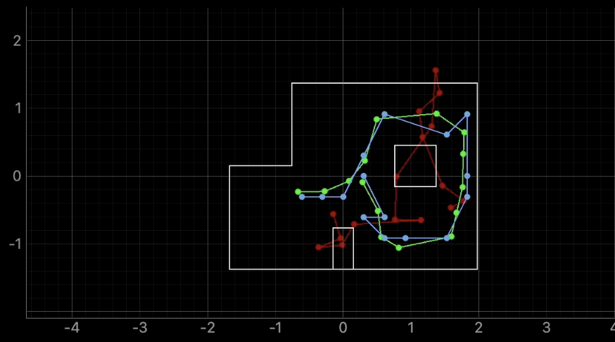
After compiling these individual functions, the simulation is copmiled with the odometry values, the Bayes Filter values, and the actual position of the stunt car in the simulation. The following is a video of the simulated running, in addition to some diagrams demonstrating a graph for the localization in the simulation:
Discussion
This lab has been a great experience to experience working with the Bayes Filter in order to continue improving stunt car localization on a grid. This proves great promise in real-world integration for better estimation of car motion. This lab was completed with Jamison Taylor, and assisted from AI tools for minor debugging.