Summary Lab #9
Lab #9 marks the first application of the ToF sensors and dynamic control for visualizing the environment around the stunt car. Whereas previous labs used singular boundary detection to determine the distance of a singular flat wall or orient the car to a specified orientation, this lab integrates orientation with linear control to determine obstacles surrounding the stunt car. The following is a closed-loop, PID-control of orientation method that is reconstructed in Jupyter Notebook to create a straight line map of the obstacles 360 degrees around the stunt car.
Lab #9 Outcomes
Obstacle Control of Stunt Car
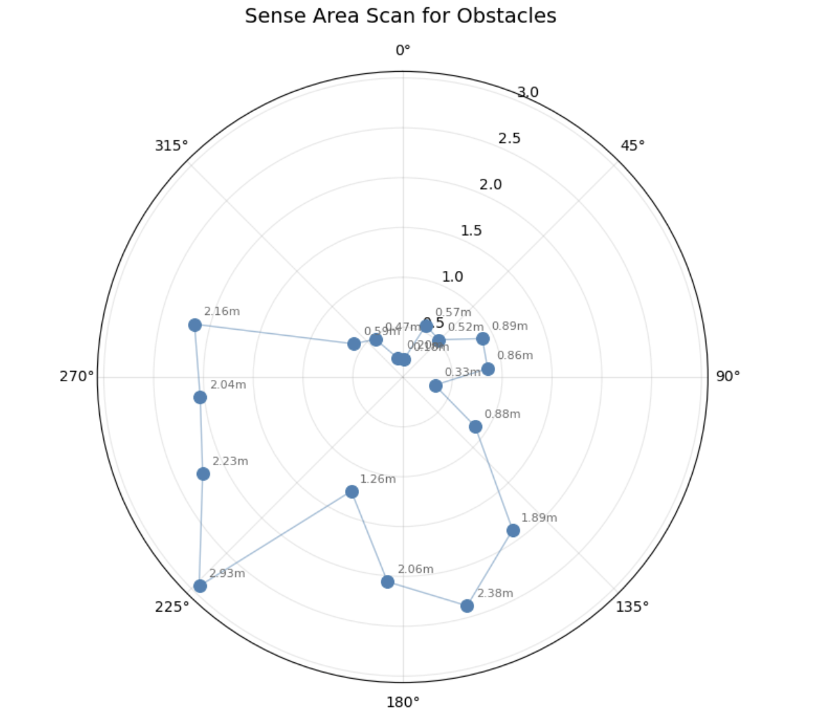
As a means for control and sampling in the open space, a PID-controlled, orientation-based method was added for determining the obstacles surrounding the stunt car. This was accomplished by first creating “sense_step()” architecture that mirrored the previous PID orientation and linear step function for control. After this function is called, an orientation PID is used to move the stunt car to 18 different points, where a ToF sensor value and yaw value are saved in individual lists. With “SENSE_TRANMISSION,” these are then transmitted from the Redboard Artemis Nano to the laptop for post-processing. The following are the respective C++ and Python scripts for computation, in addition to photos of outputs:
Jupyter Notebook (Python)
import numpy as np
import matplotlib.pyplot as plt

def plot_polar(angle_list, distance_list):
    # Debug: print lengths to see the mismatch
    # print(f"Angles: {len(angle_list)}, Distances: {len(distance_list)}")
    # print(f"Angles: {angle_list}")
    # print(f"Distances: {distance_list}")

    # Trim to the shorter list to avoid the error
    min_len = min(len(angle_list), len(distance_list))
    angle_list    = angle_list[:min_len]
    distance_list = distance_list[:min_len]

    angles_rad  = np.deg2rad(angle_list)
    distances_m = np.array(distance_list) / 1000.0
    ...

    fig, ax = plt.subplots(figsize=(7, 7), subplot_kw=dict(projection='polar'))
    fig.suptitle("Sense Area Scan for Obstacles", fontsize=14)

    ax.scatter(angles_rad, distances_m, c='steelblue', s=70, zorder=3)
    ax.plot(np.append(angles_rad, angles_rad[0]),
            np.append(distances_m, distances_m[0]),
            color='steelblue', linewidth=1, alpha=0.5)

    for i, (a, d) in enumerate(zip(angles_rad, distances_m)):
        ax.annotate(f"{d:.2f}m", (a, d), textcoords="offset points",
                xytext=(6, 6), fontsize=8, color='dimgray')

    ax.set_theta_zero_location('N')
    ax.set_theta_direction(-1)
    ax.grid(True, alpha=0.3)

    plt.tight_layout()
    plt.savefig("sense_area_polar.png", dpi=150)
    plt.show()

plot_polar(angle_list, distance_list)
Arduino Code (C++)
void loop(){
  ...
    if(sense_activate){
        unsigned long now = millis();
        if(now - ori_last_PID_time >= ori_PID_interval){
            ori_last_PID_time = now;
            sense_area_step();
        }
    }
}
...
void yaw_calculator(){
  ... (use same yaw calculator infrastructure as previous labs) ...
}

void sense_area_step() {
  if (sense_index >= 18) {
    sense_activate = false;
    ori_PID_control = false;
    analogWrite(Pin12, 0);
    analogWrite(Pin13, 0);
    analogWrite(Pin9, 0);
    analogWrite(Pin11, 0);
  }

  // Current yaw
  yaw_calculator();
  float current_yaw = yaw_deg;

  // Calculate error to target angle
  float angle_error = ori_PID_target - current_yaw;
  // Unwrap error to [-180, 180]
  if (angle_error > 180) angle_error -= 360;
  if (angle_error < -180) angle_error += 360;

  // If we're close enough to target angle, take a reading
  if (fabs(angle_error) < 5.0) {  // Within 5 degrees
    // Stop motors
    analogWrite(Pin12, 0);
    analogWrite(Pin13, 0);
    analogWrite(Pin9, 0);
    analogWrite(Pin11, 0);

    // Wait for robot to stabilize
    delay(500);

    // Take ToF reading
    float tof_reading = ToF_sensor_2.read();
    yaw_actual_points[sense_index] = tof_reading;

    // Record actual yaw angle achieved
    yaw_calculator();
    float actual_yaw = yaw_deg;

    ...

    // Move to next target
    sense_index++;
    if (sense_index < 18) {
      ori_PID_target = yaw_sample_points[sense_index];

      // Reset PID controller for new target
      ori_integral_error = 0.0;
      ori_PID_prev_error = 0.0;
      ori_prev_d = 0.0;

      Serial.print("Next target: ");
      Serial.print(ori_PID_target);
      Serial.println("°");
    }
  }
  else {
    // Not at target yet - let orientation PID run
    // Make sure orientation PID is active
    if (!ori_PID_control) {
        ori_PID_control = true;
        ori_integral_error = 0.0;
        ori_PID_prev_error = 0.0;
        ori_PID_last_time = millis();
    }

    // Compute PID output
    unsigned long now = millis();
    float dt = (now - ori_PID_last_time) / 1000.0;
    if (dt <= 0) dt = 0.001; // Guard against zero dt
    ori_PID_last_time = now;
    ori_integral_error += angle_error * dt;
    float derivative = (angle_error - ori_PID_prev_error) / dt;
    ori_PID_prev_error = angle_error;
    float output = 3 * Kop * angle_error + Koi * ori_integral_error + Kod * derivative;
    output = constrain(output, -255, 255);

    // Apply deadband
    if (output > 0 && output < 200)  output = 200;
    if (output < 0 && output > -200) output = -200;

    // Data Logging for PIDs
    if (ori_PID_counter < time_package_size) {
      ori_timestamp_value[ori_PID_counter] = now;
      ori_distance_value[ori_PID_counter]  = current_yaw;
      ori_motorPWM_value[ori_PID_counter]  = output;
      ori_proportional_value[ori_PID_counter] = angle_error;
      ori_PID_counter++;
    }

    // Drive motors in opposite directions for in-place rotation
    if (output > 0) {
      analogWrite(Pin13, (int)output);   // left reverse
      analogWrite(Pin11, (int)output);   // right forward
      analogWrite(Pin9,  0);
      analogWrite(Pin12, 0);
    } else {
      float rev = -output;
      analogWrite(Pin9,  (int)rev);      // left forward
      analogWrite(Pin12, (int)rev);      // right reverse
      analogWrite(Pin11, 0);
      analogWrite(Pin13, 0);
    }
  }
}
Example Polar Graph Output with Video
Orientation PID Controller Graphs
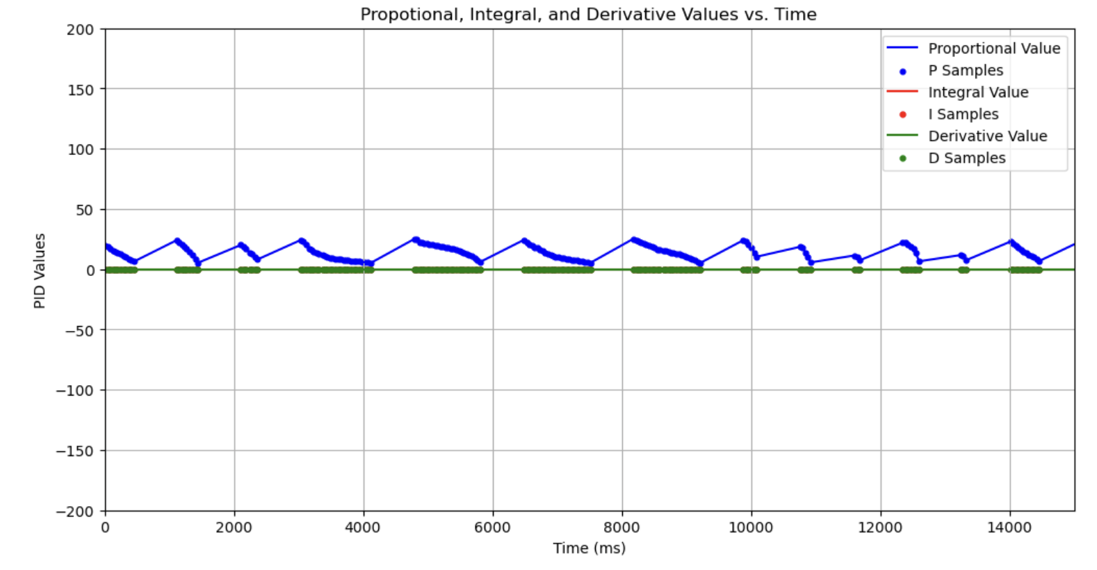
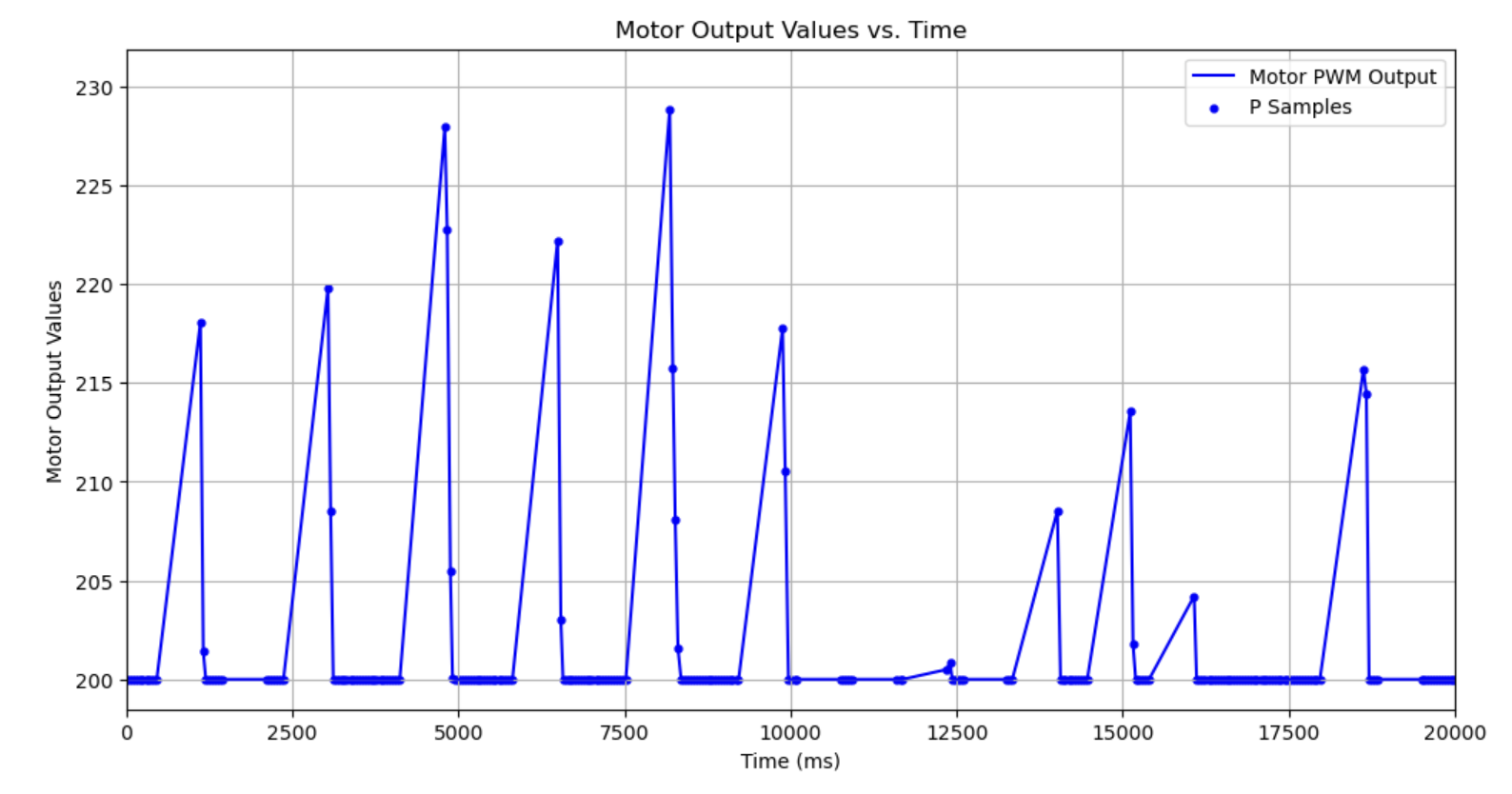
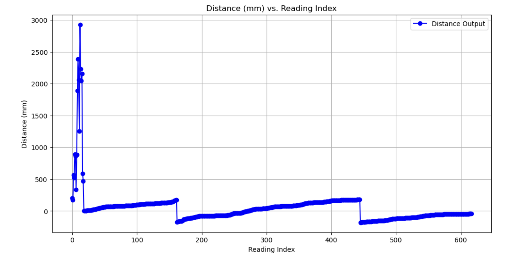
Although there appear to be some issues maintaining a perfect axis for the duration of the spin, there is consistency with the yaw degree values achieved with the PID controller. With the given code, the stunt car is commanded to move 20 degrees clockwise and take a measurement from the initial position. For the previous test computed, the mean error from the expected yaw value is 4.26 degrees, which is within the 5 degree range required for the PID to close within the stunt car script. This, in combination with the visual observations from the video, demonstrates moderate sensor drift associated with previously known limitations in the software.
Reliability of Obstacle Distances
A make-shift obstacle area is created in my lab space in order to replicate the narrow spaces of the in-class obstacle course. The following is a photo of the constructed area, the chosen orientation of the stunt car for each trial, and the respective location of each obstacle sensing case:
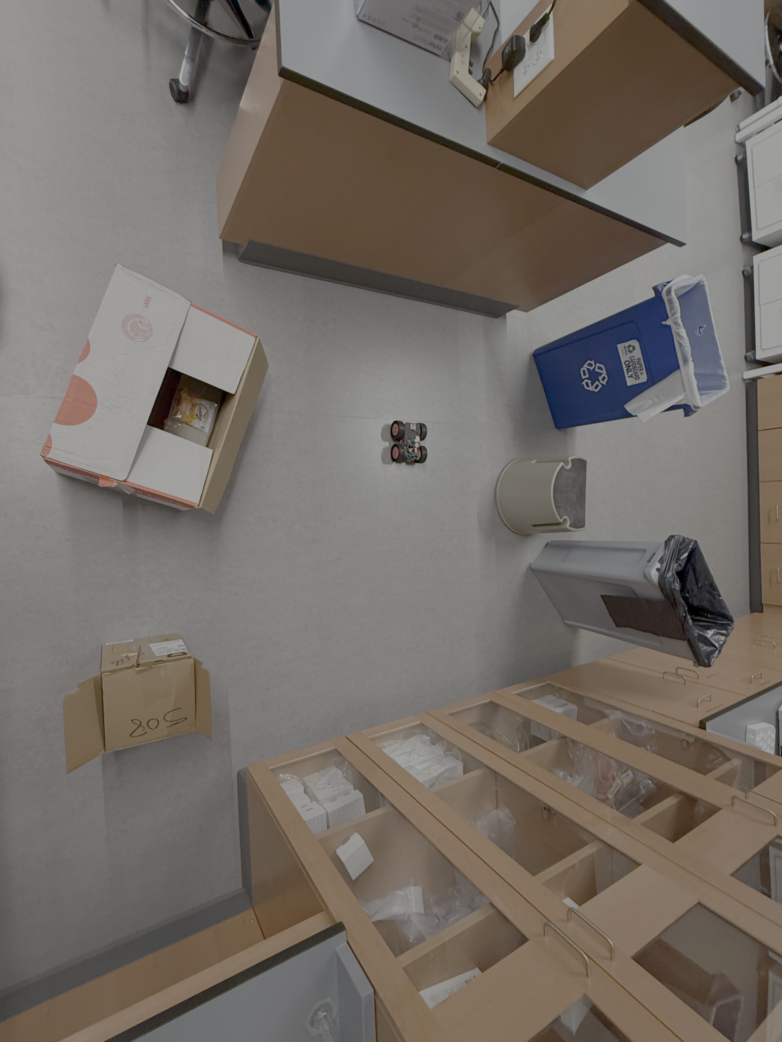
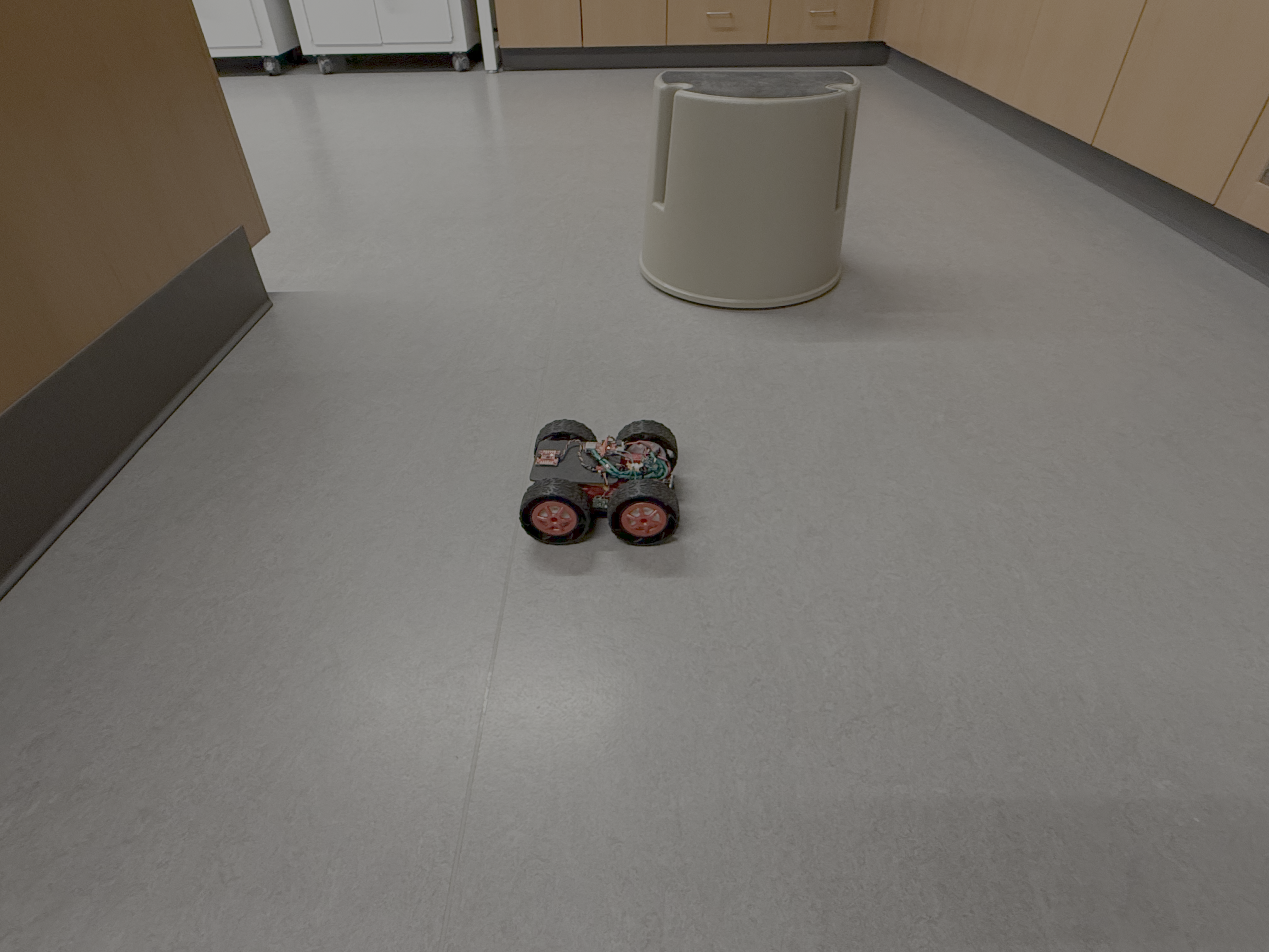
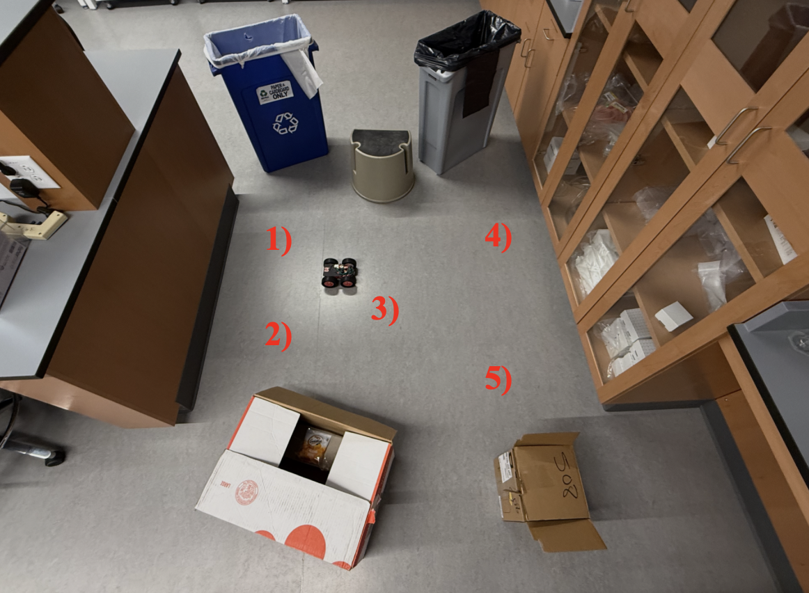
For this stage, each of the aforementioned positiosn are measured, streamed through BLE, and hand-compiled onto a singular .CSV file for clarity (screenshot below).
-
Position #1
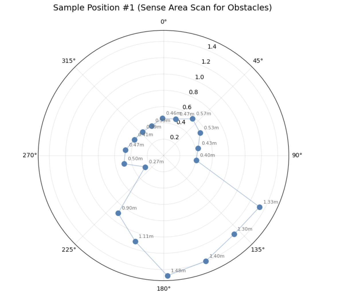
-
Position #2
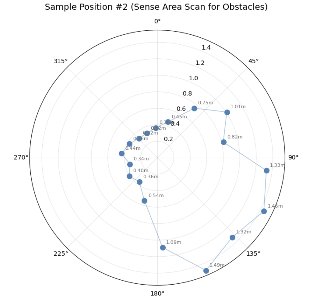
-
Position #3
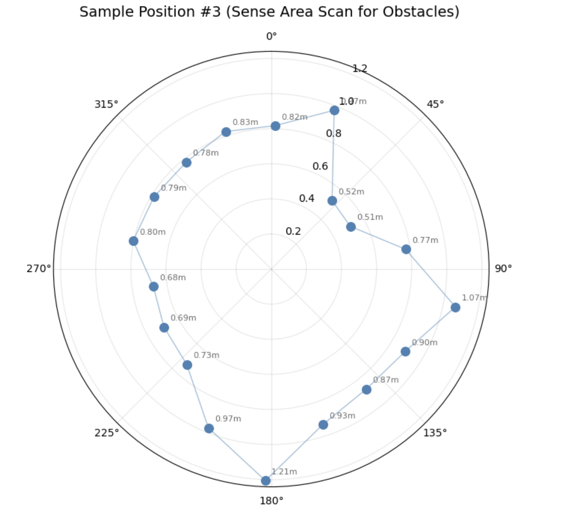
-
Position #4
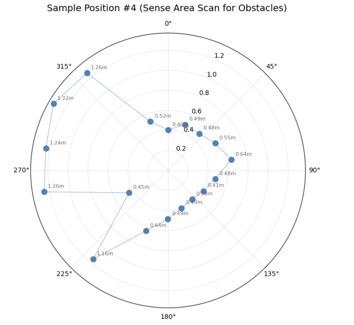
-
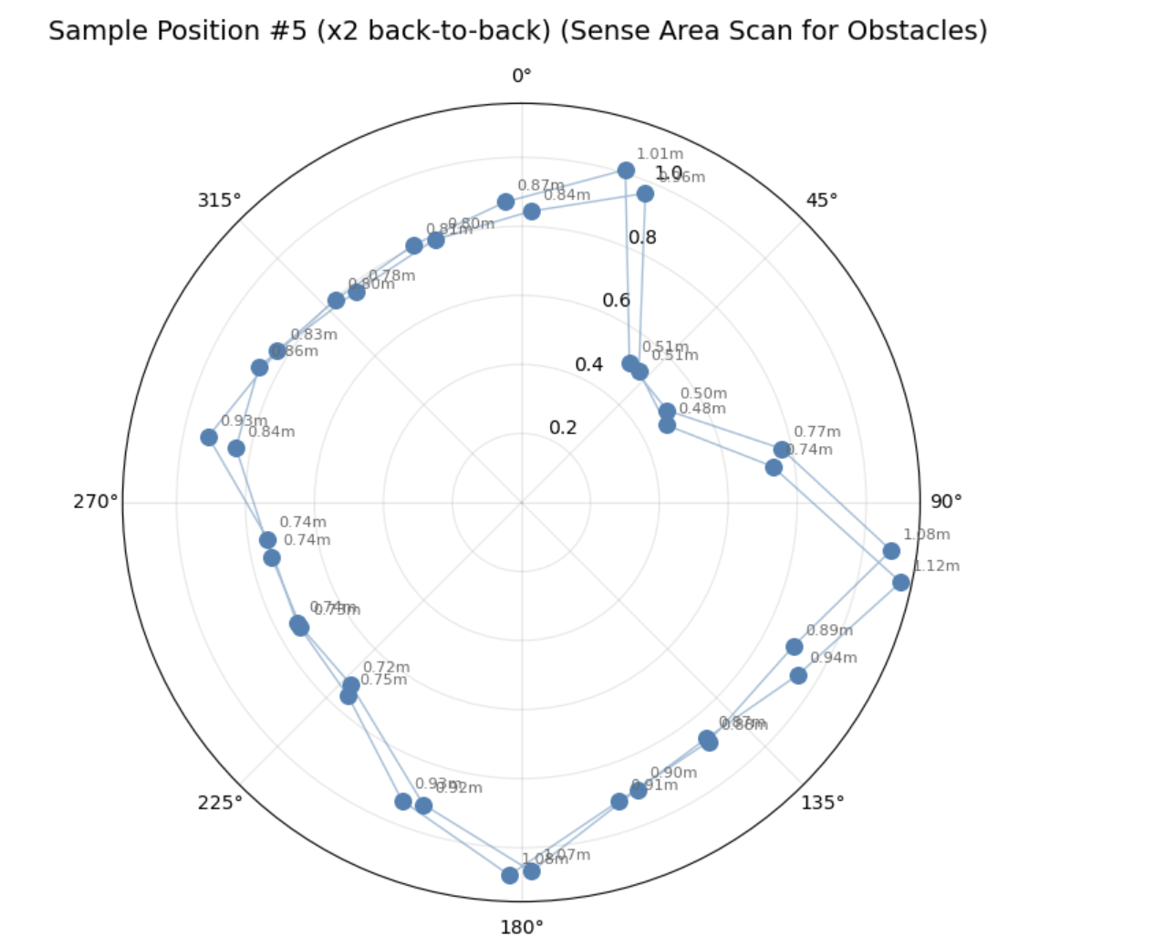
Position #5
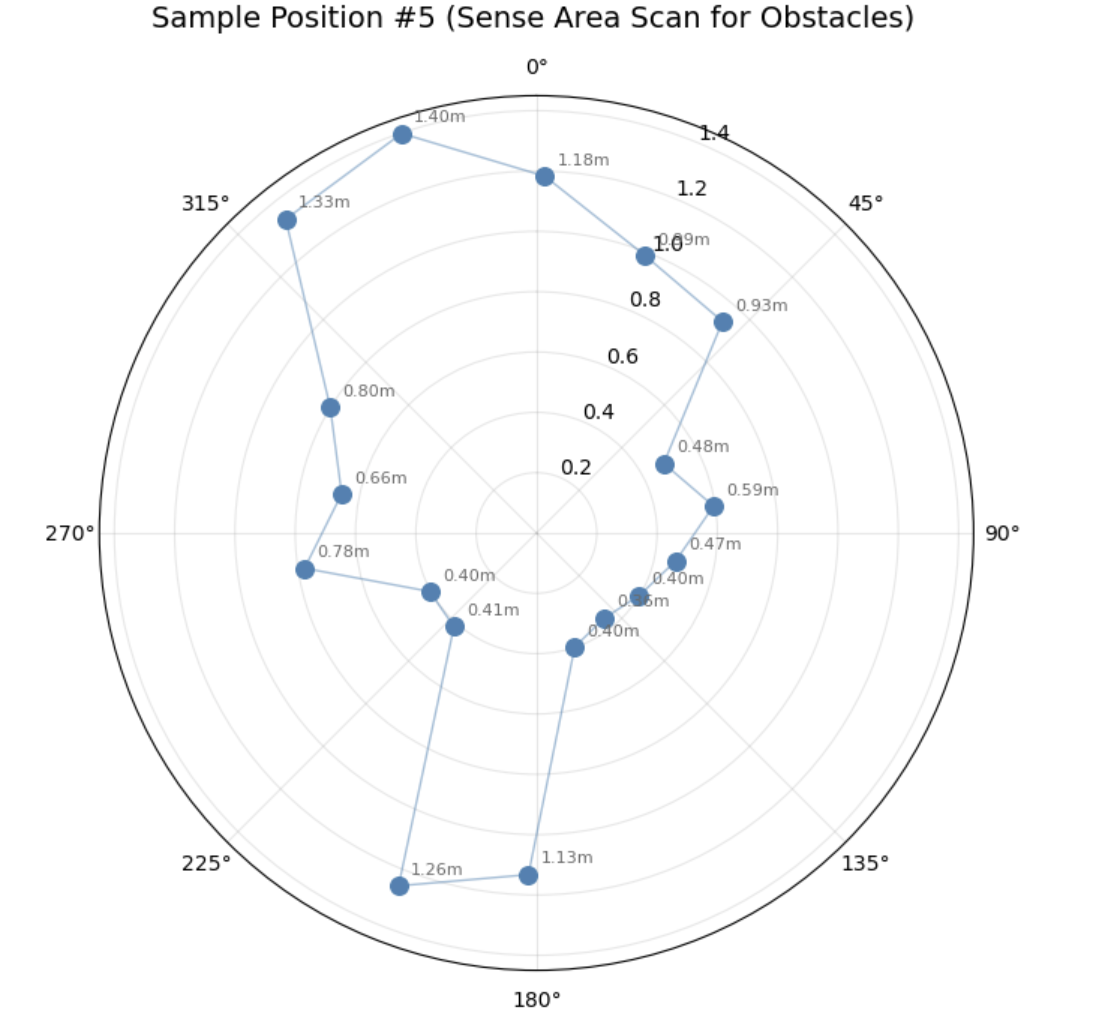
Finally, as a confirmation of the accuracy of the sensors and the method, position #3 was measured twice back-to-back. As shown in the chart, the consistency proved a high level of accuracy that provides confidence in building the model of the obstacles:
Merging Plots for Obstacle Reconstructruction
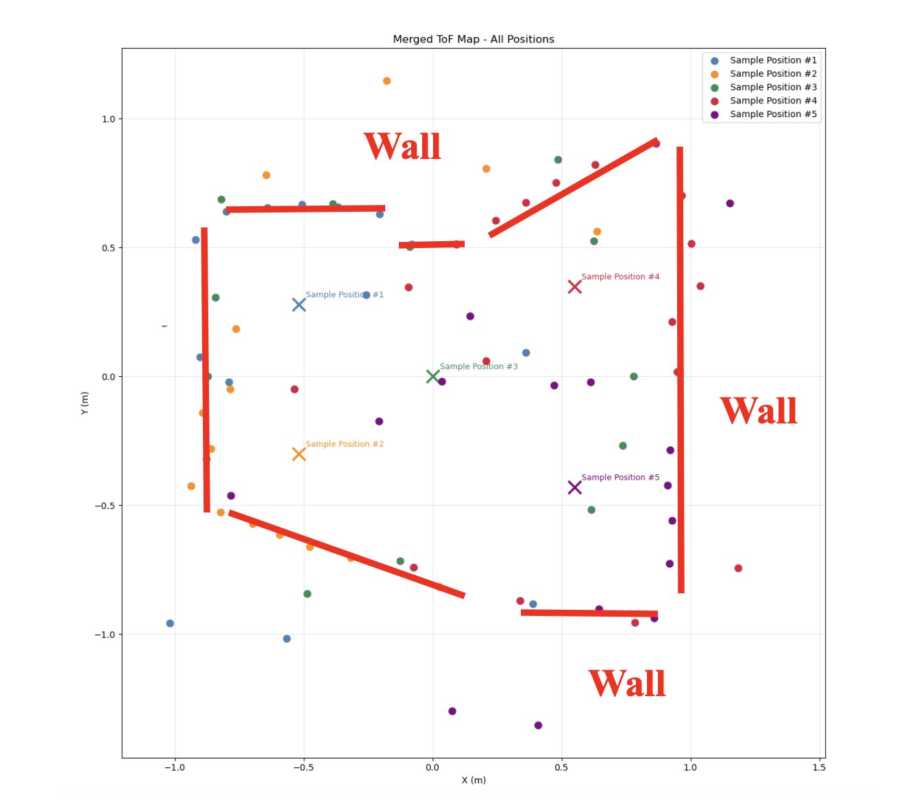
Matrix Transformation: To compute the cartesian plot of the obstacles, the stunt car yaw and ToF distances are compiled through generic transformation matricies (as discussed in class). With point #3 set as the obstacle origin (0,0), the other positions were recorded and used to set the initial positions of the point transformations. After this point, a T-matrix is used to turn the cylindrical measurement (angle and radius) into Cartesian (x and y).
With this informaiton, a basic python script is created to a) extract the information stored in an external CSV and b) post-process to provide a cartesian plot of the obstacles. Here are the outcomes from these processes:
Jupyter Notebook (Python)
position_coords = {
    "Sample Position #1": (-52 / 100,  28 / 100),
    "Sample Position #2": (-52 / 100, -30 / 100),
    "Sample Position #3": (  0 / 100,   0 / 100),
    "Sample Position #4": ( 55 / 100,  35 / 100),
    "Sample Position #5": ( 55 / 100, -43 / 100),
}
colors = ['steelblue', 'darkorange', 'seagreen', 'crimson', 'purple']

def transform_scan(angles, dists, robot_x, robot_y, start_yaw_offset, room_yaw=0):
    angles_normalized = np.array(angles) - start_yaw_offset - 180
    angles_rad  = np.deg2rad(angles_normalized)
    distances_m = np.array(dists) / 1000.0
    x_room = robot_x + distances_m * np.cos(angles_rad)
    y_room = robot_y + distances_m * np.sin(angles_rad)
    return x_room, y_room

fig, ax = plt.subplots(figsize=(12, 12))

for (label, (angles, dists)), color in zip(scans.items(), colors):
    if label not in position_coords:
        continue
    rx, ry, start_yaw = position_coords[label]
    min_len = min(len(angles), len(dists))
    angles  = angles[:min_len]
    dists   = dists[:min_len]
    x_room, y_room = transform_scan(angles, dists, rx, ry,
                                     start_yaw_offset=start_yaw,
                                     room_yaw=room_yaw)
    ax.scatter(x_room, y_room, c=color, s=60, label=label, zorder=3)
    ax.plot(rx, ry, 'x', color=color, markersize=14, markeredgewidth=2.5)
    ax.annotate(label, (rx, ry), textcoords="offset points",
                xytext=(8, 8), fontsize=9, color=color)

ax.set_xlabel("X (m)")
ax.set_ylabel("Y (m)")
ax.set_title("Merged ToF Map - All Positions")
ax.legend(loc='upper right')
ax.grid(True, alpha=0.3)
ax.set_aspect('equal')
plt.tight_layout()
plt.savefig("merged_map.png", dpi=150)
plt.show()
Line Based Map
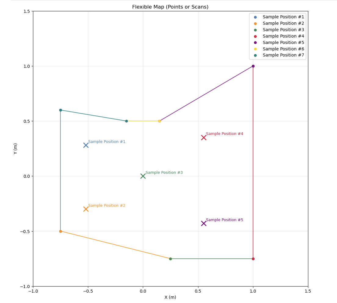
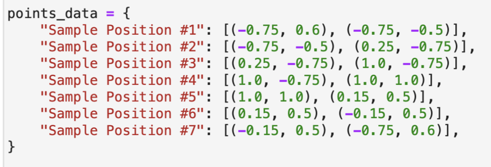
Finally, with a detailed map of the wall, this information is converted into a line-based map that includes specific coordinates that are accessible for future labs.
Discussion
This lab has been a great experience to bring in basic obstacle visualization on a 2D-plane. This is high-level considering my mechanical background, and having the opportunity to complete such a project is really exciting. Although this lab does not estimate the obstacles for the in-class apparatus, this lab still finalizes the methods that will be used to complete this estimation in the next lab. This lab was completed with Jamison Taylor, and assisted from AI tools for minor debugging.