Please Note: For transparency, this lab was submitted one day late (on 5/11 at 8:00 am) due to issues optimizing the deadband filter in addition to selecting the proper Kp, Ki, and Kd values. With this in mind, I accept the daily penalty for this specific lab and not the one week extension

Sumamry Lab #5

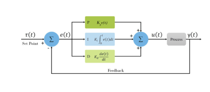
Lab #5 integrates a closed-loop feedback system for controlling the stunt car linear motion and collision detection. Where Lab #4 ended by introducing the open-loop control system for motion, Lab #5 expands by utilizing data from the Time of Flight (ToF) sensors to construct a more complex closed-loop system known as a Proportional-Integral-Derivative (PID) controller. By tuning the various gain constants for the typical PID controller framework, the stunt car is enabled with improved handling while stopping for obstacles.

Configuration

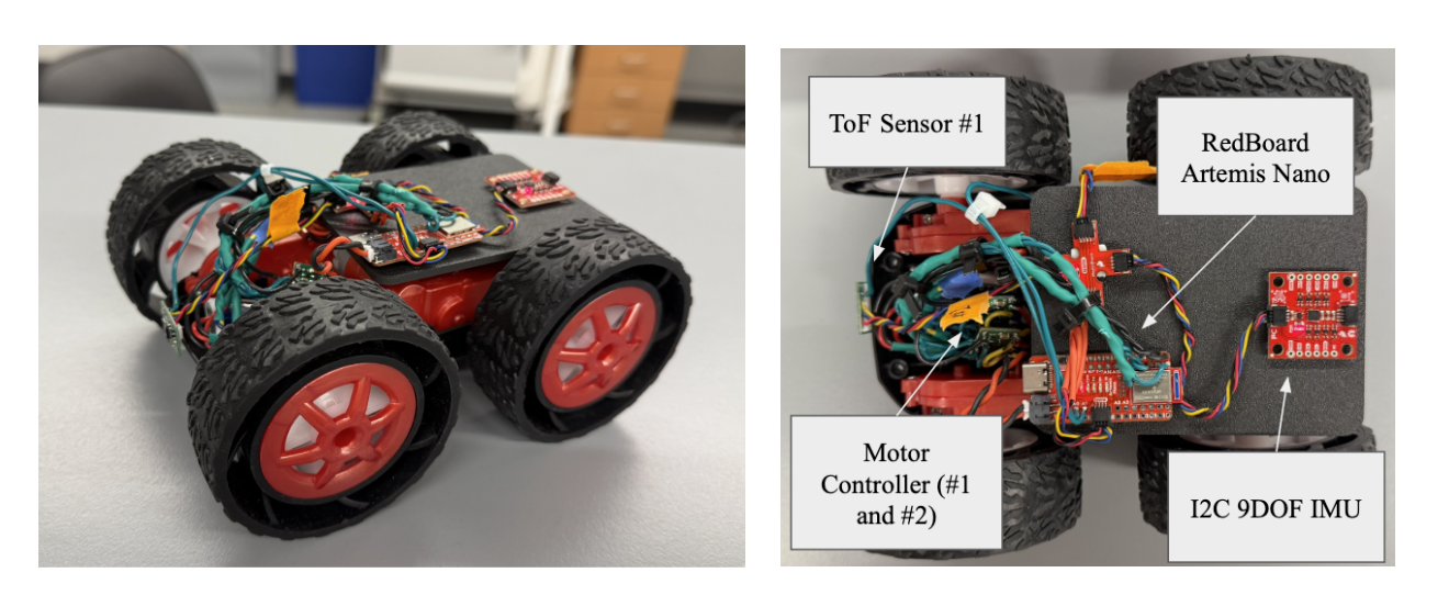
The stunt car follows the same configurations as the previous lab, including wired components, ToF locations, and overall assembly. Additionally, a custom 3D-printed plate was installed for improved mounting of the Artemis Nano, IMU sensor, and the 4-port connector. The following are images of the stunt car and sensors for the following lab:

Sending and Receiving Bluetooth for PID

The PID controller is structured by formatting the control function natively onto the RedBoard Artemis Nano and operating on-off logic with a BLE command through Python. On the Artemis Nano, the “PID_step” function is initialized in C++ for computing the instantaneous PID gains and motion:

Arduino Code (C++)

bool PID_control = false;
…
while (central.connected()) {
  write_data();
  read_data();
  if(PID_control){
      PID_step();
  }
…
void PID_step(){
// Code added later for specific PID motion
…
 if (motor_output > 0) {
   analogWrite(Pin9, motor_output * CF_Left);
   analogWrite(Pin11, motor_output * CF_Right);
   analogWrite(Pin12, 0);
   analogWrite(Pin13, 0);
 } else {
   motor_output = -motor_output;
   analogWrite(Pin12, motor_output * CF_Left);
   analogWrite(Pin13, motor_output * CF_Right);
   analogWrite(Pin9, 0);
   analogWrite(Pin11, 0);
 }
}

This function is nested into a while True loop based on the boolean value “PID_control,” which is altered externally from BLE, python commands “BEGIN_PID” and “END_PID.” In addition to these functions, “PID_GAINS” is provided to control the respective gain values, K, for the proportional, integral, and derivative components outside of beginning and ending the device:

Arduino Code (C++)

case BEGIN_PID: {
     bool Received_input = robot_cmd.get_next_value(PID_target);
     // No signal loops the previous call request
     if(!Received_input) return;
     integral_error = 0.0;
     PID_prev_error = 0.0;
     PID_last_time = millis();
     PID_counter = 0;
     PID_control = true;
     // Send Data to Python Terminal
     tx_estring_value.clear();
     tx_estring_value.append("PID Started, Target Set: ");
     tx_estring_value.append(PID_target);
     tx_estring_value.append(" mm");
     tx_characteristic_string.writeValue(tx_estring_value.c_str());
     break;
   }
  case END_PID: {
     PID_control = false;
     analogWrite(Pin12, 0);
     analogWrite(Pin13, 0);
     analogWrite(Pin9, 0);
     analogWrite(Pin11, 0);
     // Send Data to Python Terminal
     tx_estring_value.clear();
     tx_estring_value.append("PID Stopped");
     tx_characteristic_string.writeValue(tx_estring_value.c_str());
     break;
   }
case PID_GAINS: {
     bool Received_input =  robot_cmd.get_next_value(Kp)
                       && robot_cmd.get_next_value(Ki)
                       && robot_cmd.get_next_value(Kd);
     if(!Received_input) return;
     // Send Data to Python Terminal
     tx_estring_value.clear();
     tx_estring_value.append("PID Gains are Set, Kp = ");
     tx_estring_value.append(Kp);
     tx_estring_value.append(", Ki = ");
     tx_estring_value.append(Ki);
     tx_estring_value.append(", Kd = ");
     tx_estring_value.append(Kd);
     tx_characteristic_string.writeValue(tx_estring_value.c_str());
     break;
   }

Jupyter Notebook (Python)

ble.send_command(CMD.PID_GAINS, "1.2|0.0|0.05")
ble.send_command(CMD.BEGIN_PID, "304")
ble.send_command(CMD.END_PID, "")

These two functions are intended for toggling the PID function on the board, and a third function “PID_TRANSMISSION” wirelessly streams time, position, and PID values for a given package size. This streaming occurs after each of the following arrays are the size of a predetermined variable saved as “time_package_size:”

Arduino Code (C++)

case PID_TRANSMISSION: {
     for (int i = 0; i < PID_counter; i++) {
       tx_estring_value.clear();
       tx_estring_value.append("Time (ms): ");
       tx_estring_value.append(timestamp_value[i]);
       tx_estring_value.append(",");
       tx_estring_value.append("Distance: ");
       tx_estring_value.append(distance_value[i]);
       tx_estring_value.append(",");
       tx_estring_value.append("Proportional Error: ");
       tx_estring_value.append(proportional_value[i]);
       tx_estring_value.append(",");
       tx_estring_value.append("Integral Error: ");
       tx_estring_value.append(integral_value[i]);
       tx_estring_value.append(",");
       tx_estring_value.append("Derivative Error: ");
       tx_estring_value.append(derivative_value[i]);
       tx_characteristic_string.writeValue(tx_estring_value.c_str());
     }
     break;

Jupyter Notebook (Python)

time_package_size = 5000 # Consistent with Arduino
timestamp_list = []
distance_list = []
proportional_list = []
integral_list = []
derivative_list = []

def notif_callback_PID(UUID, Notif_Array):
    input_data = ble.bytearray_to_string(Notif_Array)
    processed_data = input_data.split(",")
    print(processed_data)
    timestamp_list.append(float(processed_data[0].split(": ")[1]))
    distance_list.append(float(processed_data[1].split(": ")[1]))
    proportional_list.append(float(processed_data[2].split(": ")[1]))
    integral_list.append(float(processed_data[3].split(": ")[1]))
    derivative_list.append(float(processed_data[4].split(": ")[1]))
    if len(timestamp_list) >= time_package_size:
        print("Data collection complete!")

# Start notifications
ble.start_notify(ble.uuid['RX_STRING'], notif_callback_PID)
ble.send_command(CMD.PID_TRANSMISSION, "")

Lab #4 Outcomes

P/I/D Discussion

The final closed-loop feedback controller function developed for usage during the lab is a complete PID controller controlled with the aforementioned BLE commands. The script receives data from the front ToF sensor in addition to the final distance from local objects, and calculates the respective instantaneous gain values for each of the controller components. The PID values are stored locally on the Artemis board for the “PID_TRANSMISSION” function. These were developed individually, however, are compiled and separated with comments for cohesion and clarity. The following are the major attributes of the coding structure on the Artemis Nano board:

Arduino Code (C++)

void PID_step(){
 // Setting Time Steps and variables
 float ToF_Front = ToF_sensor_2.read();
 unsigned long now = millis();
 // Derivative Time Steps for Derivative Value 
 float dt = (now - PID_last_time) / 1000.0;
 if(dt <= 0) return;
 PID_last_time = now;
 // Calculate Proportional, Integral, and Derivative Error
 float proportional_error = PID_target - ToF_Front;
 integral_error += proportional_error * dt;
 float derivative_error = (proportional_error - PID_prev_error) / dt;
 PID_prev_error = proportional_error;
 // Output Calculation
 float motor_output =  Kp*proportional_error +
                       Ki*integral_error +
                       Kd*derivative_error;
 motor_output = constrain(motor_output, -255, 255);
 // Store Values
 if (PID_counter < time_package_size) {
   distance_value[PID_counter] = ToF_Front;
   timestamp_value[PID_counter] = now;
   proportional_value[PID_counter] = proportional_error;
   integral_value[PID_counter] = integral_error;
   derivative_value[PID_counter] = derivative_error;
   PID_counter++;
 }
…
}

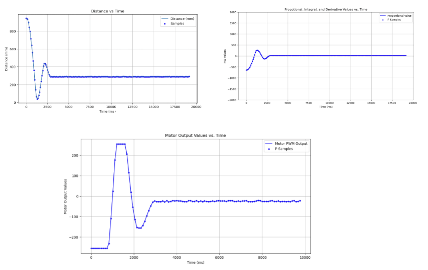
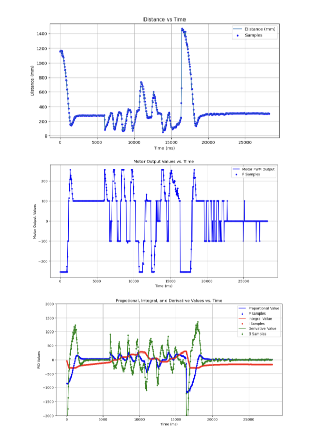
For tuning the ideal constants for common usage with the stunt car, each component of the PID controller was tuned and progressively integrated starting from proportion gain (i.e. determine P, then PI, and finally PID). The ideal distance is set to “304 mm,” or about the distance of 1 tile (marked in the videos), and motor output is reduced in half to better tune the specific gain constants (i.e. “analogWrite(PinX, motor_output/2). Finally, all distance graphs are specifically probed with the ToF sensor, thus representing ToF vs. Time next to the Motor Input vs. Time.

Proportional Gain Control (Kp)

From experimentation, proportional gain values tended to either aggressively undershoot or overshoot the ideal distance. With this in mind, values between 0.5 and 1.0 proved ideal for our given usage, however, there is still some level of adjustment for overshoot that is optimizable.

• Kp = 0.5 (Undershoot and Stalling at Lower Adjustment)

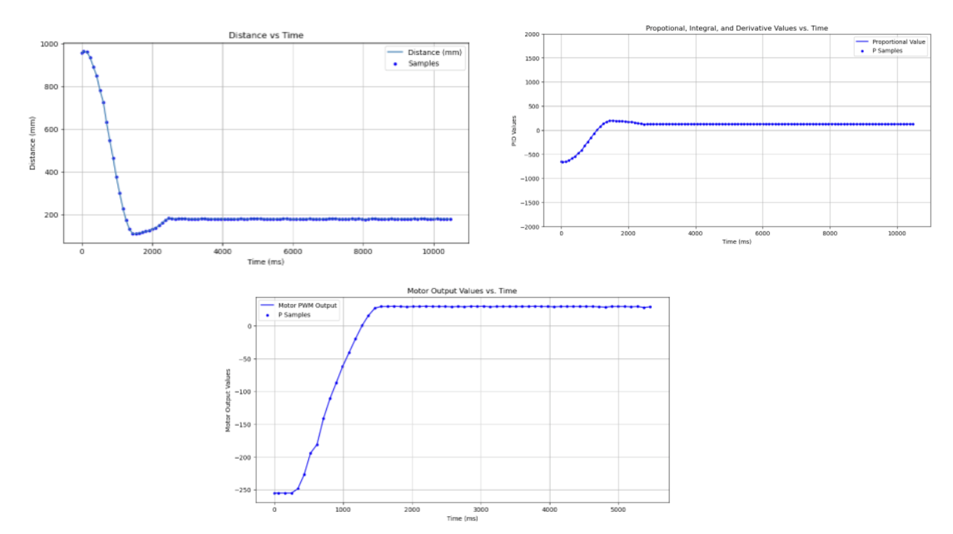
• Kp = 1.0 (Slight Overshoot)

• Kp = 1.5 (Aggressive Overshoot)

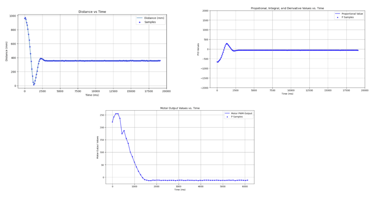
Integral Gain Control (Ki)

With Kp set to 1.0, integral gain control is implemented through a similar methodology. From experimentation, values between 0.025 and 0.075 proved strong contenders for removing the error over time and improving settling towards steady-state from just proportional gain. Ki = 0.05 provided the best steady-state at ~310 mm during experimental testing. These calibrations were done with Kp = 1.0 to highlight the effect of changing Ki in general.

• Ki = 0.025 (Moderately Deviated Value)

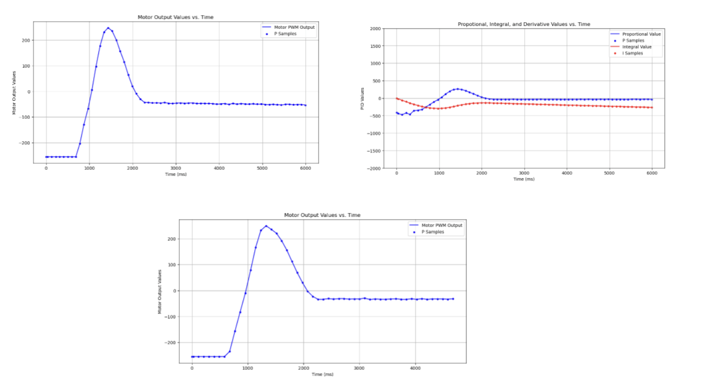
• Ki = 0.5 (Close Final Steady-State Value)

• Ki = 0.075 (Slightly Higher Steady-State Value)

Additional motor controller attributes were added such as a deadband filter to prevent motor stalling at low outputs and anti-windup.

Deadband Filter

if (motor_output > 0 && motor_output < 40) motor_output = 40;
if (motor_output < 0 && motor_output > -40) motor_output = -40;

Anti-Windup

integral_error = constrain(integral_error, -300, 300);

Derivative Gain Control (Kd)

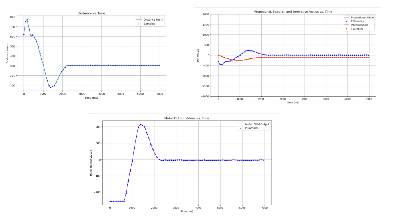
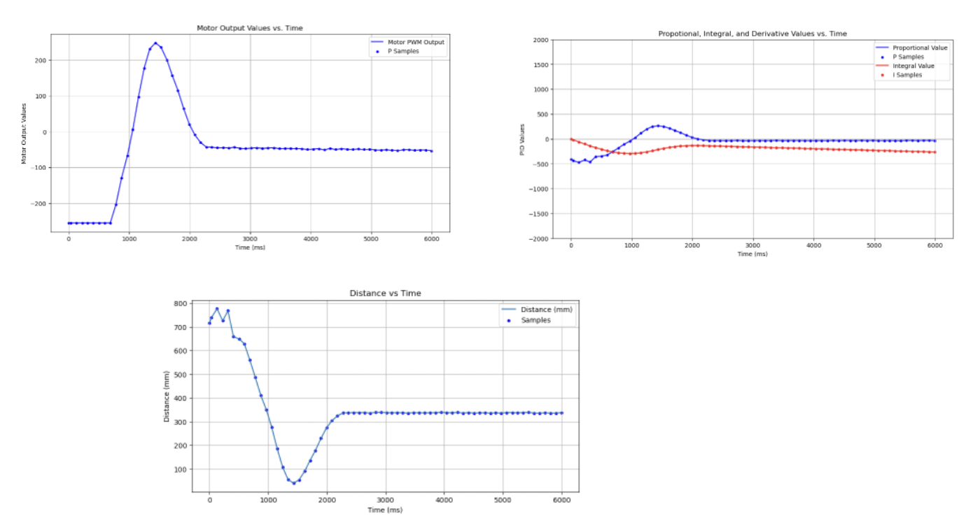
Finally, from additional testing and tweaking of all the values, Kd = 0.12 is determined as a strong final gain constant for the derivative control. After selecting Kp = 1.0, Ki = 0.05, and Kd = 0.12, a final trial is conducted to analyze the efficacy of the total gain values. Here are the results from this trial:

Video with Readjustment

Outputs from Total Testing with Kp = 1.0, Ki = 0.05, and Kd = 0.12

Range and Sampling Time

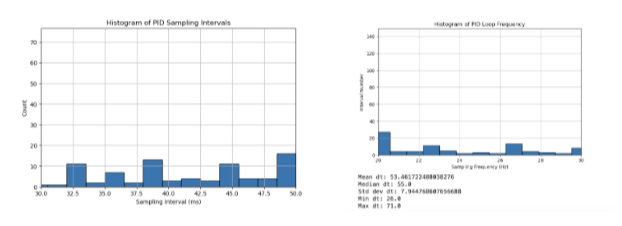
As established in Lab #3, the ToF sensors for this specific stunt car configuration is set to the medium-range mode, which has proved effective for sensing objects in a large room as seen with the following use cases. The sensors are set to the minimum timing budget of the ToF sensors which is about every 20 ms or about a 50 Hz sampling frequency, however, there is bottlenecking occurring with the Serial.print statements that are leading to a message rate between 30 - 60 ms, with incredibly high-variability. The following is an overview of the histogram method for comparing the sampling/ message rate:

Jupyter Notebook (Python)

final_time = norm_time[len(norm_time)-1] / 1000
print(f"{len(timestamp_list)} messages were received")
print(f"Estimated message transfer rate is ~ {len(timestamp_list)/final_time} msgs/s")
print(f"Estimated message transfer rate is ~ {len(timestamp_list)/final_time} Hz")
…
# Histogram of dt
plt.figure(figsize=(8,5))
plt.hist(dt, bins=30, edgecolor='black')
plt.xlabel("Sampling Interval (ms)")
plt.ylabel("Count")
plt.title("Histogram of PID Sampling Intervals")
plt.grid(True)
plt.show()

# Histogram of frequency
freq = 1000.0 / dt
plt.figure(figsize=(8,5))
plt.hist(freq, bins=30, edgecolor='black')
plt.xlabel("Sampling Frequency (Hz)")
plt.ylabel("Count")
plt.title("Histogram of PID Loop Frequency")
plt.grid(True)
plt.show

Histogram of Time Intervals

Linear Extrapolation

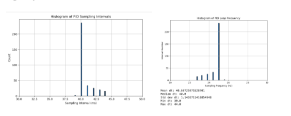
Finally, to improve performance for receiving ToF data, a linear extrapolation subscript was implemented in the “PID_step” function. This checks for the availability of data, and extrapolates expected distance based on previous distance/ speed to improve processing performance. For testing accuracy and reliability of setting sampling rate, 25 Hz was set as the message sending rate, which is togglable through BLE. The following is the specific code snippet implemented in the function:

Arduino Code (C++)

unsigned long last_pid_time = 0;
const unsigned long PID_INTERVAL = 25; //ms
if(PID_control){
         unsigned long now = millis();
         if(now - last_PID_time >= PID_interval){
           last_PID_time = now;
           PID_step();
         }
       }
...
void PID_step(){
 // Setting Time Steps and variables
 unsigned long now = millis();
 float dt = (now - PID_last_time) / 1000.0;
 if(ToF_sensor_2.checkForDataReady()){
   ToF_Front = ToF_sensor_2.read();
 } else if(PID_counter > 2){
   float x1 = distance_value[PID_counter-2];
   float x2 = distance_value[PID_counter-1];
   float t1 = timestamp_value[PID_counter-2]/1000;
   float t2 = timestamp_value[PID_counter-1]/1000;
   float extrapolated_slope = (x2-x1) / (t2-t1);
   ToF_Front = x2 + extrapolated_slope*((now/1000)-t2)
 } else{
   ToF_Front = ToF_sensor_2.read();
 }
…

Histogram of Time Intervals with Linear Extrapolation

Discussion

This lab was a great chance to integrate PID knowledge from previous System Dynamics classes into real-world, robotic application. The tuning for the individual gain controllers for proportional, integral, and derivative constants provided a strong in-depth analysis for their individual contributions to motor dynamics. This lab was completed with Jamison Taylor, assisted from AI tools for minor debugging, and referenced against Tyler Wisnieski’s GitHub page for comparing effective code structures.