Summary (1A and 1B)
Lab #1 is a basic introduction of the Artemis Nano board and interacting with the Arduino IDE, through both direct connection and BLE. In Lab #1A, the Artemis board is configured for a MacBook (M2 Pro) and basic scripts are executed including Blink, Serial, AnalogRead, and Microphone Output. In Lab #1B, bluetooth communication is established through Jupyter Notebook to wirelessly communicate with the Artemis board, and basic verification testing scripts are conducted to confirm a reliable connection.
Lab 1A
Configurations
Prior to beginning, some steps were required to configure my computer for communicating with the Artemis board. This included installing the Artemis library for the preinstalled ArduinoIDE, downloading the CH340 Driver, and configuring particular settings for the bootloader. After completing this, the ArduinoIDE could recognize and burn scripts.

Outcomes
Multiple tests were conducted to verify the Artemis Nano board is operating as expected, as shown in the videos below:
- Test #1 - Blink: “Blink” demonstrates the board’s ability to control an on-board LED with HIGH and LOW controls
- Test #2 - Serial: “Serial” demonstrates the board’s ability to communicate through the Serial Monitor and echo back commands types through the computer
- Test #3 - AnalogRead: “AnalogRead” demonstrates the board’s ability to read from the die temperature sensor on the Apollo3 microcontroller
- Test #4 - Microphone Output: “Microphone Output” demonstrates the board’s ability to recognize external frequencies with the built-in microphone, and print out the loudest frequency on the Serial Monitor. During the video, I am trying to whistle an F# (~1480 Hz)
Lab 1B
Configurations
Prior to beginning the next lab, additional steps were completed to create the virtual environments required for running bluetooth for the Artemis Nano board. This included multiple steps, first including downloading python, creating the FastRobots_ble virtual environment with Python, and uploading the “ble_robot_1.4” codebase into the project directory. After this, the “ble_arduino.ino” script is loaded onto the board to extract the Artemis MAC address, generate a new UUID in Jupyter Notebook, and update the “connection.yaml” file with the new MAC address in the project directory. There are smaller steps beyond this to produce the first demo for bluetooth capabilities, but for brevity these are omitted.
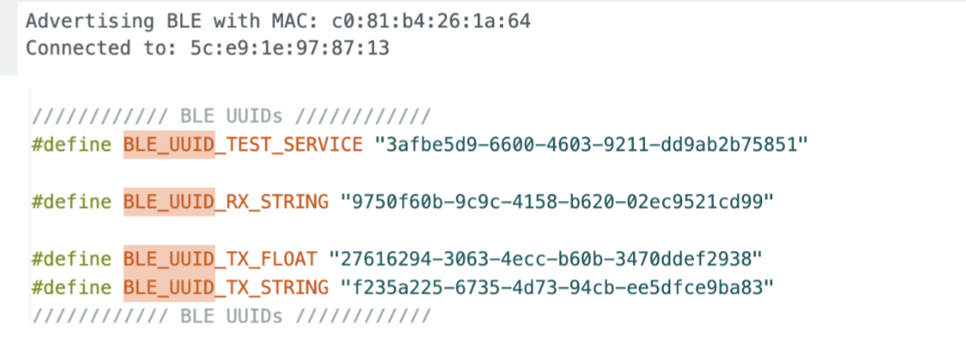
Now that the BLE environment has been initialized, the codebase creates a two-way wireless Bluetooth Low Energy (BLE) communication channel designed for low power devices. BLE operates with a central-peripheral system, where the peripheral (i.e. the Artemis Nano board) advertises itself to the central (i.e. Main Computer) and provides structured information as services and characteristics. Each piece of information has a unique UUID which enables the computer to read and write characteristics, in addition to subscribing for updates. With this, a publish-subscribe system is accessible for wireless controlling the Artemis Nano and receiving sensor data through Bluetooth.
Outcomes
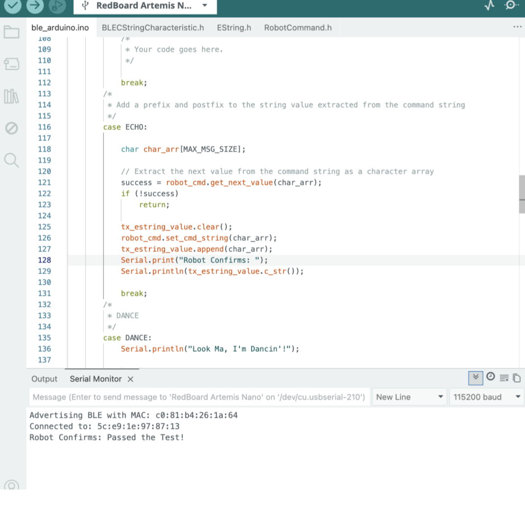
- Function #1 - ECHO: Jupyter Notebook sends a command through the “Echo()” function that includes “Passed the Test!”, and prints out “Robot Confirm: Passed the Test!” in the Serial Monitor.
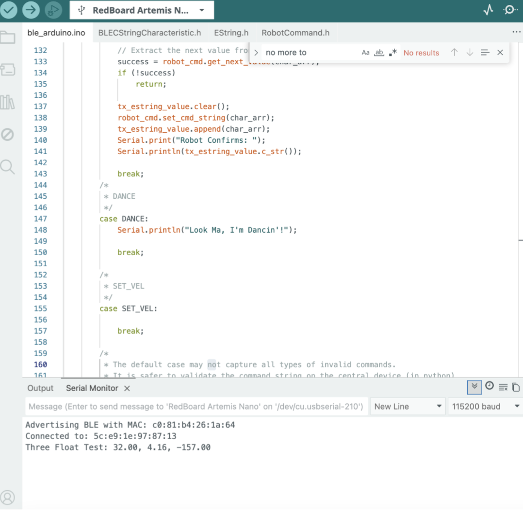
- Function #2 - SEND_THREE_FLOATS: Jupyter Notebook sends a command through the “Send_Three_Floats()” function to read out three values (“32 | 4.16 | -157”) and outputs the reformatted results into the Serial Monitor as “Three Float Test: 32.00, 4.16, -157.00.”
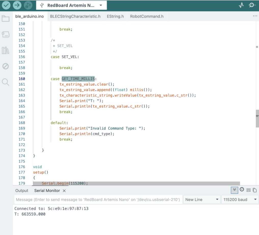
- Function #3 - GET_TIME_MILLIS: Jupyter Notebook sends a command through the “GET_TIME_MILLIS()” function that calls for the time recorded on the Artemis clock and prints the “T: Timestamp” in the Serial Monitor.
-
Function #4 - NOTIF_CALL: In Jupyter Notebook, the function “Notif_Call” is created to obtain and print the timestamp for accessing the specific microcontroller with the commands. Compiling is done to confirm no Python-based errors, none of which were flagged.
-
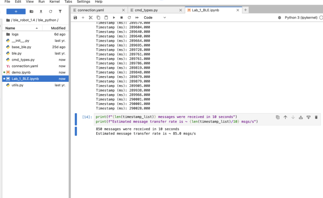
Function #5 - MESSAGE_SPEED: In Jupyter Notebook, use the “Notif_Call” function in combination with “start_notify” function to create a finite list of timestamps dictated by “Message_Speed()” function on the Artemis board. Over ten seconds, the Artemis board sends notifications unconstrained and computes the average data transfer rate and prints in the Jupyter Notebook terminal. From testing different variations, the highest effective data transfer rate was capped around 100 messages per second, where anything beyond this point would cause crashing for the system. I would recommend that for future use, a buffer should be added to prevent exceeding this limit and continue smooth operation.
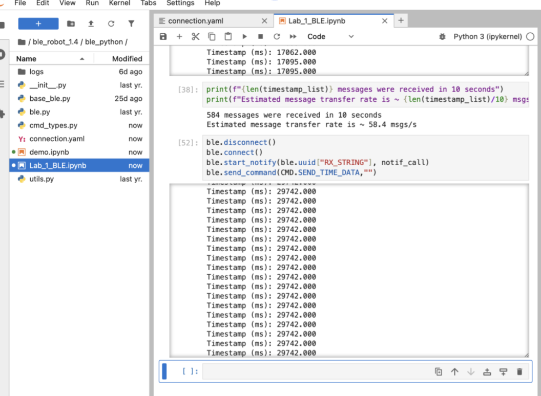
- Function #6 - SEND_TIME_DATA: Jupyter Notebook sends a command through the “Send_Time_Data()” function that calls the Artemis board to store a set amount of data and stream the information back to the Jupyter Notebook terminal.
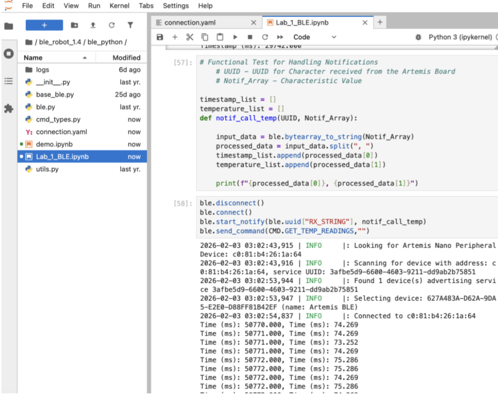
- Function #7 - GET_TEMP_READINGS: Jupyter Notebook sends a command through the “GET_TEMP_READING()” function that compiles the timestamp and datapoint for temperature through the die temperature sensor on the Artemis board, sends the information to Jupyter Notebook, and recompiles the information for printing on the Jupyter Notebook terminal.
Relevant Arduino Code Snippets
enum CommandTypes
{
    ...
    MESSAGE_SPEED,
    SEND_TIME_DATA,
    GET_TEMP_READINGS,
};
case SEND_THREE_FLOATS:
    float three_float_array[3];
    for (int i = 0; i < 3; i++) {
        success = robot_cmd.get_next_value(three_float_array[i]);
        if (!success) {
            return;
        }
    }
    Serial.print("Three Float Test: ");
    Serial.print(three_float_array[0]);
    Serial.print(", ");
    Serial.print(three_float_array[1]);
    Serial.print(", ");
    Serial.println(three_float_array[2]);
case GET_TIME_MILLIS:
    tx_estring_value.clear();
    tx_estring_value.append((float) millis());
    tx_characteristic_string.writeValue(tx_estring_value.c_str());
    Serial.print("T: ");
    Serial.println(tx_estring_value.c_str());
    break;
case MESSAGE_SPEED:{
    // Find the average over 10 seconds
    unsigned long init_time = millis();
    int sample_time = 10000; // Units (ms)
    while(10000 > millis() - init_time){
        tx_estring_value.clear();
        tx_estring_value.append((float) millis());
        tx_characteristic_string.writeValue(tx_estring_value.c_str());
    }
    break; }
case SEND_TIME_DATA:{
    // 2) Record timestamps
    for (int i = 0; i < time_package_size; i++){
        timestamp_array[i] = (float) millis();
    }

    // 3) Communicate array to Jupyter Notebook
    for (int i = 0; i < time_package_size; i++){
        tx_estring_value.clear();
        tx_estring_value.append((float) timestamp_array[i]);
        tx_characteristic_string.writeValue(tx_estring_value.c_str());
    }
    break; }
case GET_TEMP_READINGS:{
    unsigned long init_time = millis();
    for (int i = 0; i < time_package_size; i++){
        timestamp_array[i] = (float) millis();
        temperature_array[i] = (float) getTempDegF();
    }
    for (int i = 0; i < time_package_size; i++){
        tx_estring_value.clear();
        tx_estring_value.append("Time (ms): ");
        tx_estring_value.append((float) timestamp_array[i]);
        tx_estring_value.append(", Time (ms): ");
        tx_estring_value.append((float) temperature_array[i]);
        tx_characteristic_string.writeValue(tx_estring_value.c_str());
    }
    break; }
Relevant Python Code Snippets
...
ble.send_command(CMD.ECHO, "Passed the Test!")
ble.send_command(CMD.SEND_THREE_FLOATS, "32|4.16|-157")
ble.send_command(CMD.GET_TIME_MILLIS, "")
ble.start_notify(ble.uuid["RX_STRING"], notif_call)
ble.send_command(CMD.MESSAGE_SPEED,"")
ble.start_notify(ble.uuid["RX_STRING"], notif_call)
ble.send_command(CMD.SEND_TIME_DATA,"")
timestamp_list = []
temperature_list = []
def notif_call_temp(UUID, Notif_Array):
    input_data = ble.bytearray_to_string(Notif_Array)
    processed_data = input_data.split(", ")
    timestamp_list.append(processed_data[0])
    temperature_list.append(processed_data[1])
    print(f"{processed_data[0]}, {processed_data[1]}")
Discussion
Throughout this lab, I became familiar with the basic infrastructure for sending and receiving information through direct and wireless connections. This ranges from configuring the Artemis board, burning normal scripts, communicating with the Serial Monitor, creating the infrastructure for a virtual environment through Jupyter Notebook, and sending data through BLE. Major challenges included software blocks associated with using an Apple computer during the initial configuration, but beyond this, all future steps faced little issues. Overall, this lab was a strong start towards building the digital infrastructure for assembling the robots in the upcoming labs.