Summary Lab #2
Lab #2 initializes the SparkFun 9DOF IMU, specifically the accelerometer and gyroscope chips, for deriving stunt car orientation. For this lab, classes and functions from the provided SparkFun example scripts are merged with elements from the Lab #1’s BLE files to continuously stream relevant information. This information is both observed through USB-C direct connection on the Serial Monitor for basic understanding, and through Jupyter Notebook for noise reduction and complex post-processing.
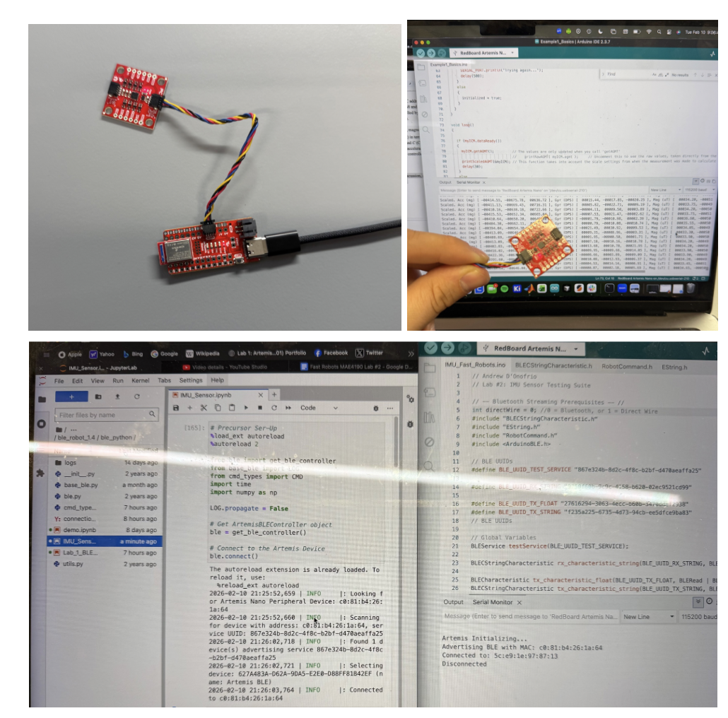
Configurations
The Redboard Artemis Nano is connected to the SparkFun 9DOF IMU Breakout Board with a QWIIC connector and powered through the USB-C connection. For this lab, both USB direct wire connection and bluetooth are completed workflows for displaying outputs from the IMU set-up, and photos will vary based on the post-processing requirements. For quick affirmation, output from the Serial Monitor is provided, but otherwise, BLE in Jupyter Notebook is provided.
AD0_VAL Application
AV0_VAL selects the I2C address for the connected IMU board, since IMU-20948 has two possible I2C addresses (0x68 and 0x69). For the functions in the provided Sparkfun Arduino file, the I2C address is controlled by the ADR jumper being open (1) or closed (0) which is indicated in the AD0_VAL variable.
The sensors record the acceleration, gyroscope, magnetometer, of pitch, roll, yaw (9 outputs/ data points) and temperature (1 additional datapoint) in terms of mgs (milli-g-force, mm/s^2), DPS (degrees-per-second, theta/s), uT (microTeslas), and C (Celsius). These are 3D vectors (with positive and negative values) indicating the respective acceleration and orientation of the specific IMU, with sampling rate and Serial Monitor Output controlled by the Sparkfun functions and code.
Lab #2 Outcomes
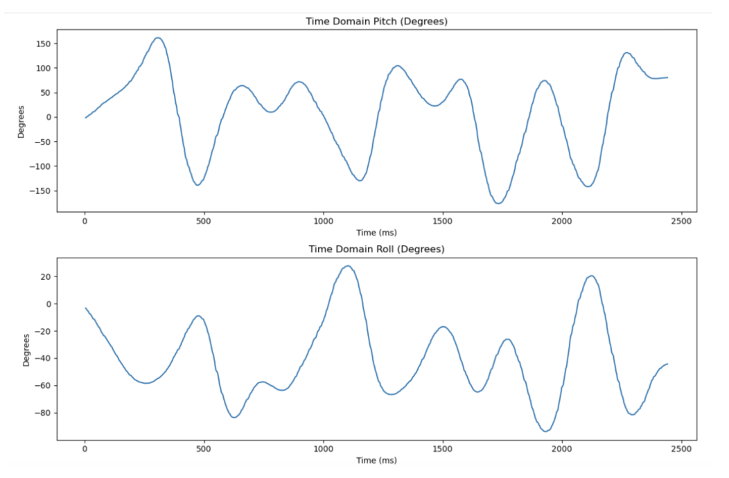
Accelerometer (Pitch and Roll from -90, 0, 90)
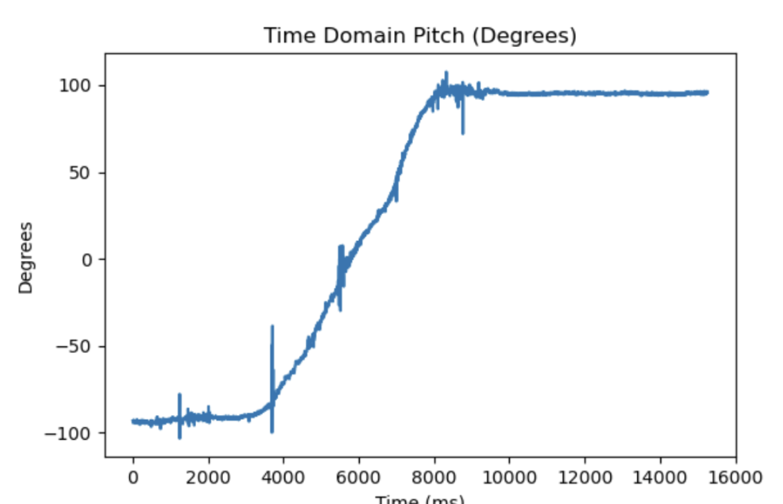
Pitch Data
Roll Data
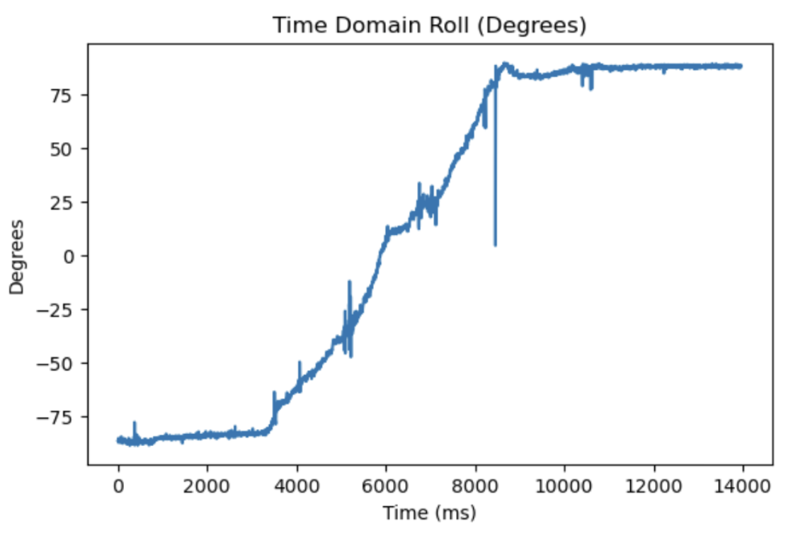
- Accuracy: While the accelerometer has high-accuracy, the precision is lower considering the high-frequency noise propagating in the time-dependent graph. For both pitch and roll, there are spikes in the even motion occurring, indicating high-sensitivity in the sensors that picks up high-frequency, low-amplitude signals.
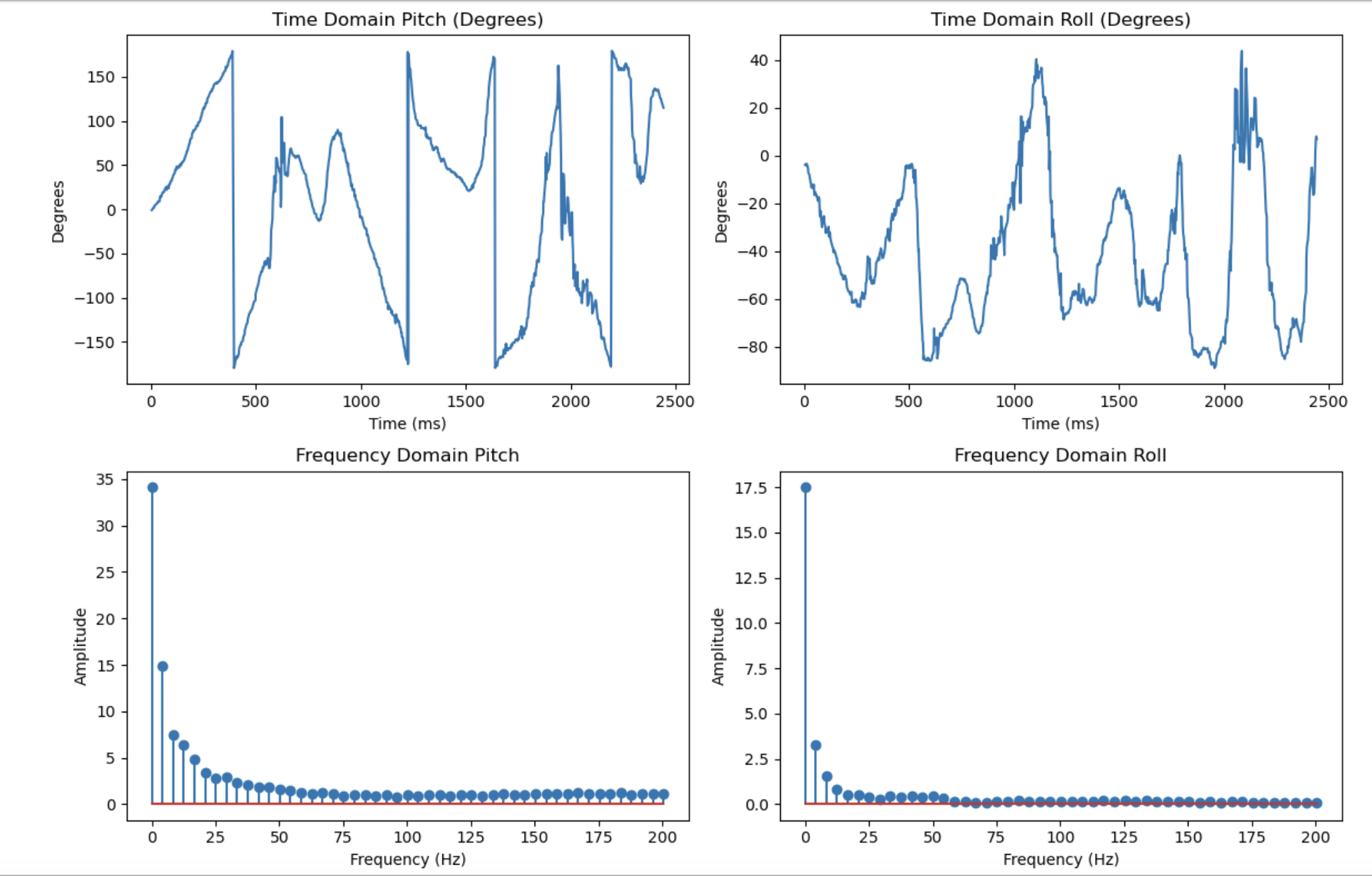
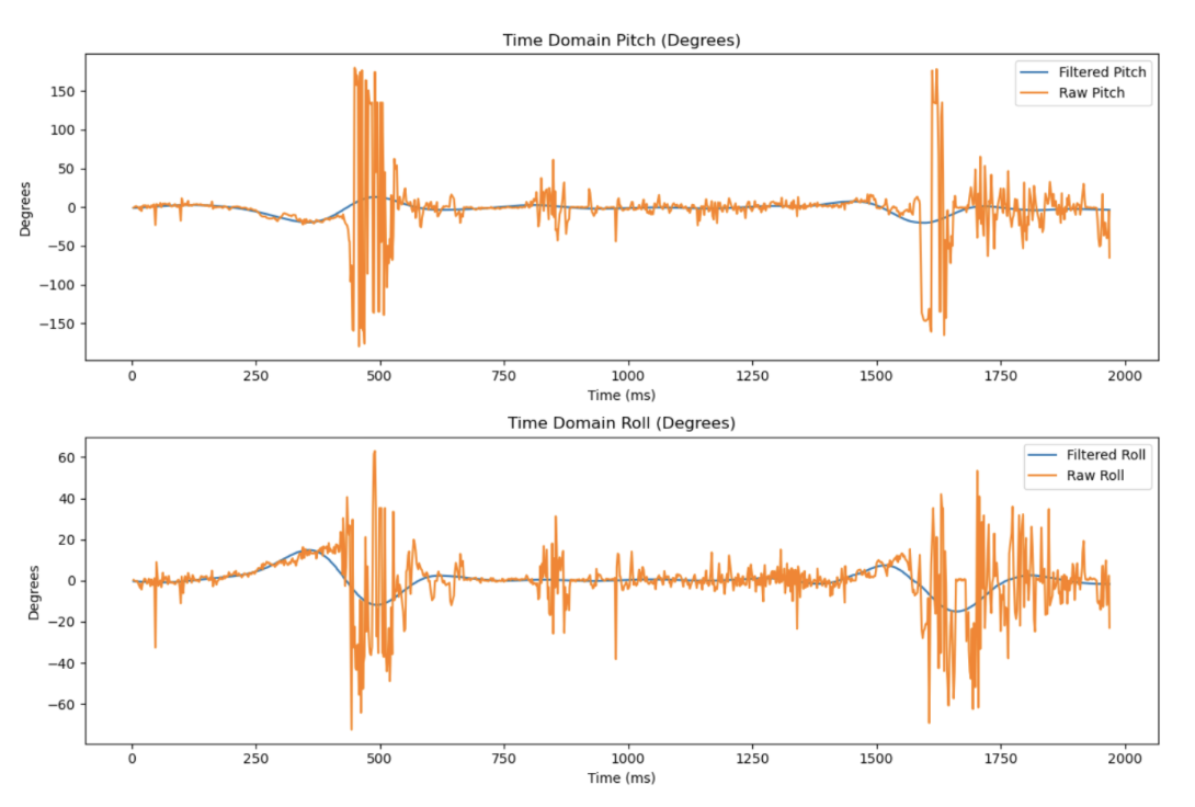
- Low-Pass Filtering with FFT: The following is a side-by-side of the pre-processed time-dependent motion graphs from the accelerometer, a fast fourier transform (FFT) of the pre-processed data, and the post-processed data with the low-filter applied in Python. As shown below and from the previous section, the raw accelerometer data is especially noisy. A digital low-pass filter is implemented in order to remove unnecessarily detailed artifacts recorded during data collection and smooth the dataset. With high-amplitude signals up to around 3 Hz, I implemented a 5 Hz low-pass filter. Disregarding the DC-offset demonstrated in the dataset, the ~3 dB point below the maximum amplitude is at about 3-4 Hz, and with 5 Hz indicating a smoothing factor of alpha = 0.072, 5 Hz proves a sound cut-off frequency.
Pre-processed Time-Dependent Motion Graphs and Fast Fourier Transforms (FFTs)
Post-Processed Time-Dependent Motion Graphs with 5 Hz Low-Pass Filter
Pre-Processed and Post-Processed Time-Dependent Motion Graphs

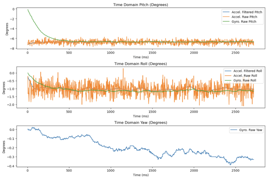
Here is an additional analysis of the low-pass filter with vibrational noise generated from bashing the IMU sensor against the table. As seen, the vibrational artifacts are not preserved with this cut-off frequency.
Relevant Code Structure
void accelerometerIMUs(ICM_20948_I2C *sensor) {
  // Assigning Acceleration Values
  float accX_est = sensor->accX() / 1000.0;
  float accY_est = sensor->accY() / 1000.0;
  float accZ_est = sensor->accZ() / 1000.0;

  // Estiamted Roll and Pitch
  // Radians
  float accel_roll = atan2(accY_est, accZ_est);
  float accel_pitch = atan2(-accX_est, sqrt(accY_est*accY_est + accZ_est*accZ_est));
  // Degrees
  accel_roll = accel_roll * 180.0 / M_PI;
  accel_pitch = accel_pitch * 180.0 / M_PI;
  // Output
  SERIAL_PORT.print(" Pitch (deg): ");
  SERIAL_PORT.print(accel_pitch, 2);
  SERIAL_PORT.print(",");
  SERIAL_PORT.print(" Roll (deg): ");
  SERIAL_PORT.println(accel_roll, 2);
  delay(100);
}

void gyroscopeIMUs(ICM_20948_I2C *sensor) {
  unsigned long now = millis();

  if (last_time == 0) {
    last_time = now;
    return;
  }

  float dt = (now - last_time) / 1000.0;
  last_time = now;

  float gyrX_est = sensor->gyrX();
  float gyrY_est = sensor->gyrY();
  float gyrZ_est = sensor->gyrZ();

  gyro_roll  += gyrX_est * dt;
  gyro_pitch += gyrY_est * dt;
  gyro_yaw   += gyrZ_est * dt;
  SERIAL_PORT.print("Pitch (deg): ");
  SERIAL_PORT.print(gyro_pitch, 2);
  SERIAL_PORT.print(",");
  SERIAL_PORT.print(" Roll (deg): ");
  SERIAL_PORT.print(",");
  SERIAL_PORT.print(gyro_roll, 2);
  SERIAL_PORT.print(" Yaw (deg): ");
  SERIAL_PORT.println(gyro_yaw, 2);
}
case GET_ALL_IMU_READINGS: {
unsigned long init_time = millis();
float alpha = 0.8; // Complementary filter coefficient
for (int i = 0; i < time_package_size; i++) {
unsigned long now = millis();
if (myICM.dataReady()) {
myICM.getAGMT();
}
// --- Accelerometer angles ---
float accX = myICM.accX() / 1000.0;
float accY = myICM.accY() / 1000.0;
float accZ = myICM.accZ() / 1000.0;
float roll_acc = atan2(accY, accZ) * 180.0 / M_PI;
float pitch_acc = atan2(-accX, sqrt(accY*accY + accZ*accZ)) * 180.0 / M_PI;
// --- Gyroscope integration ---
static unsigned long last_time_local = 0; // inside loop, static to keep value
float dt;
if (last_time_local == 0) {
dt = 0.0;
} else {
dt = (now - last_time_local) / 1000.0;
}
last_time_local = now;
float gyrX_est = myICM.gyrX();
float gyrY_est = myICM.gyrY();
float gyrZ_est = myICM.gyrZ();
// Integrate gyro
if (i == 0) {
est_gyro_roll[i] = gyrX_est * dt;
est_gyro_pitch[i] = gyrY_est * dt;
est_gyro_yaw[i] = gyrZ_est * dt;
} else {
est_gyro_roll[i] = est_gyro_roll[i-1] + gyrX_est * dt;
est_gyro_pitch[i] = est_gyro_pitch[i-1] + gyrY_est * dt;
est_gyro_yaw[i] = est_gyro_yaw[i-1] + gyrZ_est * dt;
}
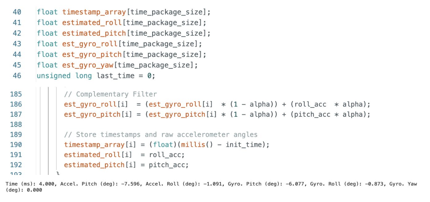
// Complementary Filter
est_gyro_roll[i] = (est_gyro_roll[i] * (1 - alpha)) + (roll_acc * alpha);
est_gyro_pitch[i] = (est_gyro_pitch[i] * (1 - alpha)) + (pitch_acc * alpha);
// Store timestamps and raw accelerometer angles
timestamp_array[i] = (float)(millis() - init_time);
estimated_roll[i] = roll_acc;
estimated_pitch[i] = pitch_acc;
}
...
Gyroscope
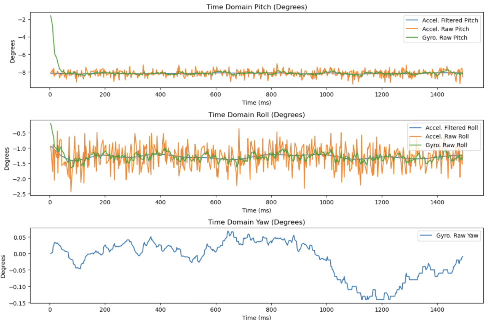
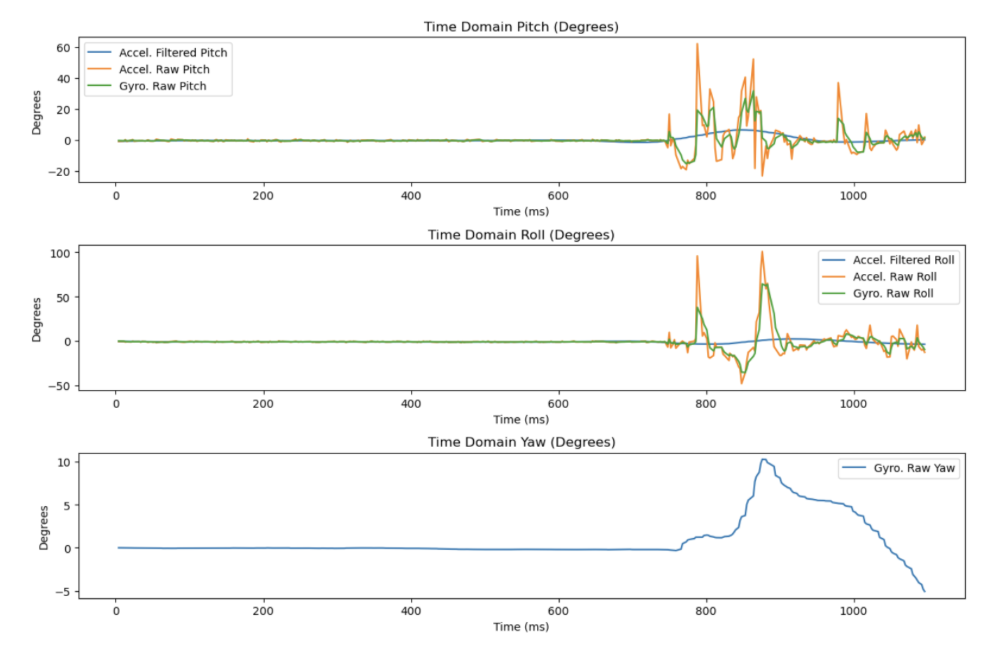
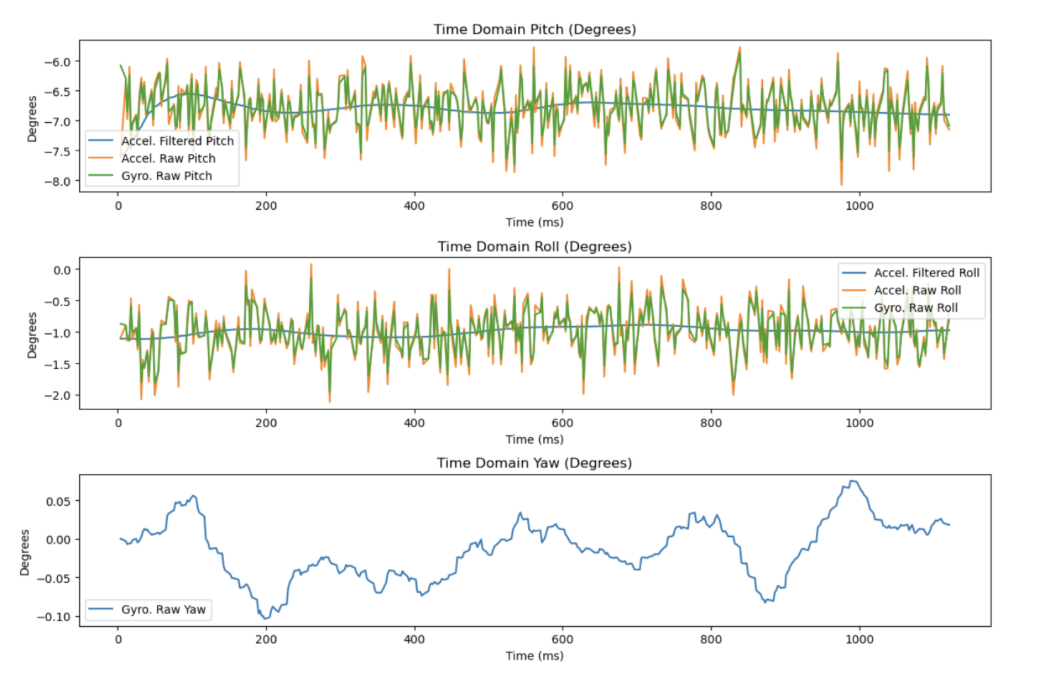
After setting up the accelerometer chip with direct wire and BLE, the gyroscope is connected and continuously streamed to compare the angular displacement between the two chips. Gyroscope data is formulated with the time-step equations provided in class, leading to noticeable drift within the gyroscope data over time. Accelerometer pitch and roll (raw and filtered), in addition to gyroscope pitch, roll, and yaw (raw) are below.
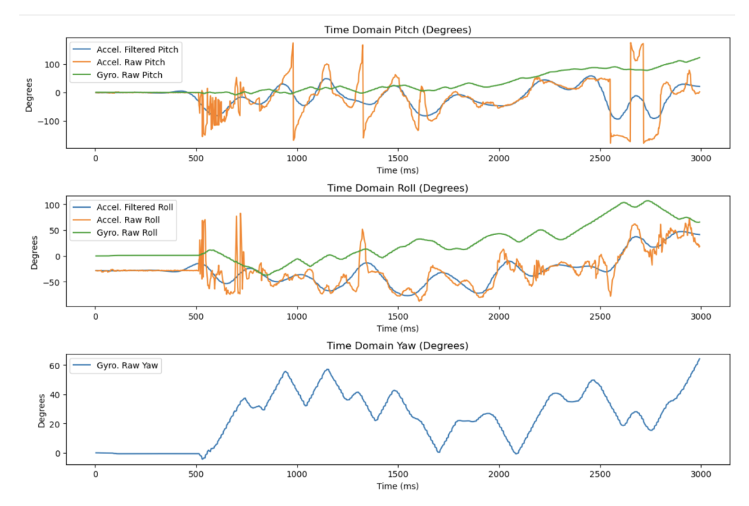
With the complementary filter (formula seen below), the approximation for pitch and roll visualized in the graphs demonstrates greater accuracy over a set response time. Similar to a logarithmic function approaching a specific value, the gyroscope approximation improves in accuracy with greater data (as a general rule). Across different alpha values, the higher the value, the greater the fit for the approximated gyroscopic data is to the raw accelerometer data. From this, I will centralize on an alpha value of ~0.5.
- Alpha = 0.02:
- Alpha = 0.2:
- Alpha = 0.4:
- Alpha = 0.8:
Sample Data
With the bluetooth arrangement and removing all print statements, the Artemis board transmits data with a sampling frequency of ~350 Hz to ~400 Hz. Sizes of arrays were preallocated with the variable “time_pacakge_size” for 5000 to stream about 10-12 seconds worth of data. My method involves storing all the IMU data into separate accelerometer and gyroscope arrays, and then streaming the data over after a set timeframe by looping through the arrays. These are then reassembled in the Jupyter Notebook.
- Speed of Sampling
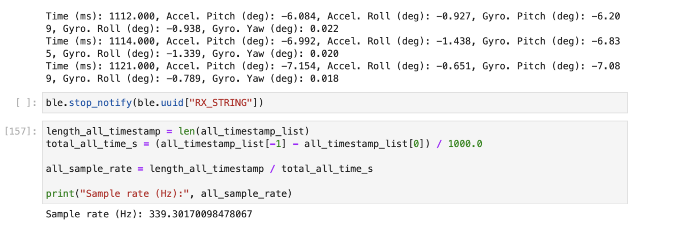
- Time-Stamped IMU Data
There are numerous considerations for these arrays, specifically regarding the number of arrays, type allocation, and the Artemis memory. Each data point is saved in separate arrays in order to better isolate for post-processing in Python and data points are saved as floats for precision while timestamps are saved as unsigned integers for efficiency. With all of this in mind, this should allow for efficient operation and prevent the Artemis Nano RAM from being congested with saving temporary values.
Over 5 seconds of IMU Data on BLE
Here is a video demonstrating the Artemis arrays transmitted via bluetooth and printed in Jupyter Notebook for ~11 seconds of data:
Record a Stunt
Here is a video of a stunt done with the car:
The stunt car responds efficiently to inputs from the controller, accelerates suddenly, and handles dynamically. Unlike standard RC Cars, the stunt car is able to perform tank spins (360-degree spins) since the left and right tires are independently powered. This additionally contributes to the tight turning and aggressive response to input parameters from the controllers. Although normal cars would be impacted by the reduced torque and handling, these attributes are outside our scope and are effective tradeoffs.
Discussion
Overall, Lab #2 provided the opporutnity to establish a useful conneciton between the peripheral sensors and the BLE environrmnet. This will be the building blocks for future labs and creating the infrastructure for large-scale data processing in Python and C++.