Lab 7: Kalman Filtering

Please Note: This lab was submitted one day after the deadline (the night of 3/24) after troubleshooting in lab

Summary Lab #7

Lab #7 is an opportunity for integrating a Kalman Filter for the motion of the stunt car, optimizing the process for estimating the distance and velocity attributes of the stunt car with additional information regarding uncertainty and noise. With these additional metrics included into the estimation method for these attributes, this provides better insight on the inputs and observations of the robot. In this lab, the Kalman Filter is integrated both in the Jupyter Notebook (through Python) and the Artemis Nano Board (through C++) and improved by performing basic drives into a wall.

Configuration

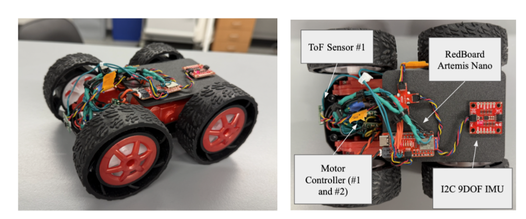
The stunt car configuration is still the same from all previous labs, including wired components, ToF locations, and overall assembly (with the 3D printed plates). The following is an image of the stunt car and sensors for the lab:

An additional BLE case was implemented on the Artemis Nano Board to act as a control system for the ramming action and the Kalman Filter. These are controlled with new BLE functions and a basic “notify” Python function in Jupyter Notebook:

Arduino Code (C++)

case KALMAN:{
     float output = 128;   // 50% Maximum Motor Output
     float start_time = millis();
     float dist = ToF_sensor_2.read();
     // Drive Forward
     while(dist > 50){
       dist = ToF_sensor_2.read();
       float now = millis();


       analogWrite(Pin12, output * CF_Left);
       analogWrite(Pin13, output * CF_Right);
       analogWrite(Pin9, 0);
       analogWrite(Pin11, 0);
	// Additional Control Code
     }
     analogWrite(Pin12, 0);
     analogWrite(Pin13, 0);
     analogWrite(Pin9, 0);
     analogWrite(Pin11, 0);
     break;

Jupyter Notebook (Python)

def notif_callback_K(UUID, Notif_Array):
    input_data = ble.bytearray_to_string(Notif_Array)
    processed_data = input_data.split(",")
    print(processed_data)
    timestamp_list.append(float(processed_data[0].split(": ")[1]))
    motorPWM_list.append(float(processed_data[1].split(": ")[1]))
    distance_list.append(float(processed_data[2].split(": ")[1]))

Lab #7 Outcomes

Altogether, the lab report is primarily a walkthrough of the first implementation of the stunt car running into the wall with the Kalman Filter in Python, followed by the same action but with the Kalman Filter implemented on the robots. Provided is the code snippets, process outcomes, and general steps for creating these

Kalman Filter in Python (External)

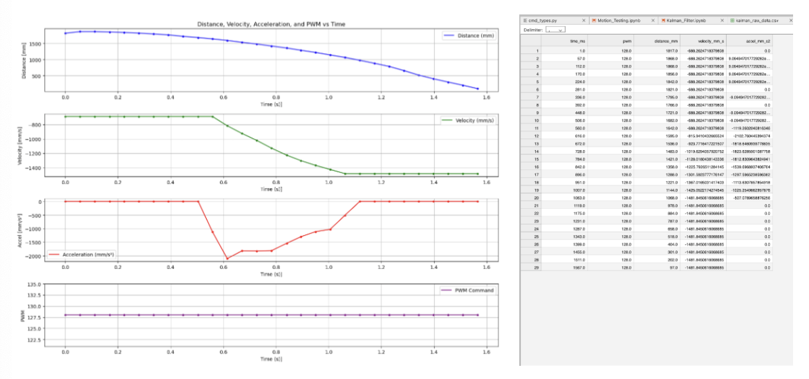
A basic test case was conducted running the car with 50% motor speed into the wall and continuously streaming the data through BLE.

Estimate Drag and Momentum: With motor input at 50%, an initial wall ramming test was conducted in order to determine the viability of the post-processing methods for velocity and acceleration. This method yielded an estimated steady-state (90%) velocity at 1367.02 mm/s and a d/m value at 0.0864, which appeared reasonable given the use case. The following charts and .CSV files of the raw data were developed from this testing:

Jupyter Notebook (Python)

# Data Preparation
df["time_s"] = (df["time_ms"] - df["time_ms"][0]) / 1000.0
step_pwm = max(df["pwm"])
df["u_norm"] = df["pwm"] / step_pwm

# Interpolation
t = df["time_s"].values
u = df["u_norm"].values
z = df["distance_mm"].values
u_interp = np.interp(t, t, u)

# Velocity
df["vel"] = np.gradient(df["distance_mm"], df["time_s"])
window = 20
df["vel_smooth"] = df["vel"].rolling(window, center=True).mean()
df["vel_smooth"] = df["vel_smooth"].fillna(method="bfill").fillna(method="ffill")

# Acceleration
df["accel"] = np.gradient(df["vel_smooth"], df["time_s"])

# Additional Code to Plot All in separate graphs

Initialize KF (Python): Following the steps provided by the lab instructions, the A, B, and C matrices for the Kalman Filtering process are computed in the Jupyter Notebook, Python environment.

PHOTO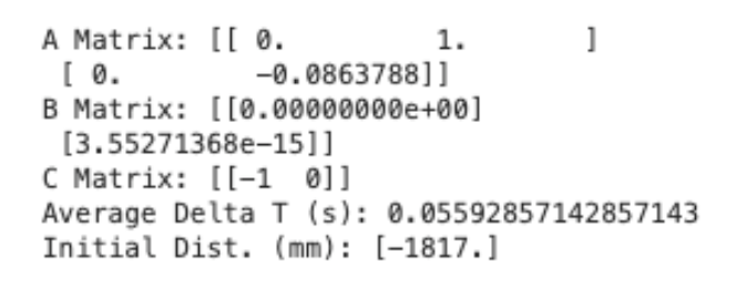 Lab_1_1

Basic Kalman Filter: With these attributes processed, the actual Kalman Filter is processed and graphed in conjunction with the process and sensor noise covariance values. For this specific usage, the following standard deviations (with covariance) are chosen:
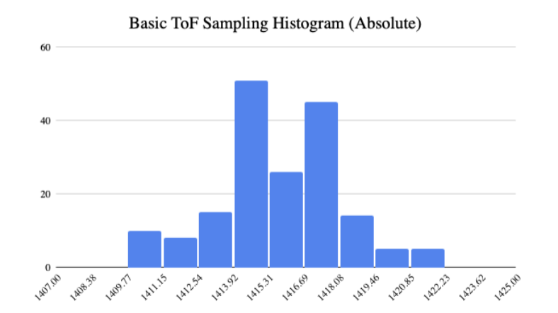
1. ToF Sensors: ~2.5 mm (6.25 mm), determined through an experimental method where the car is at a fixed distance of ~1400 mm, sampled every 50 ms. From this experiment, the standard deviation from the mean datapoint was estimated to be ~2.5 mm
1. Velocity Process: ~340.00 mm/s, calculated with a basic Python script that estimated the standard deviation of the velocity estimate after 1 second (with the formula demonstrated in class lecture)
Jupyter Notebook (Python)
```
dt = np.diff(t)
dt_mean = np.mean(dt)
steps_per_second = 1.0 / dt_mean
sigma_2 = np.sqrt(Sigma_u[1, 1])   # velocity process std [mm/s]
vel_std_1s = sigma_2 * np.sqrt(steps_per_second)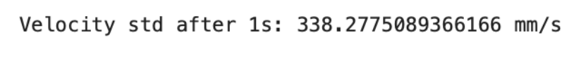
```
1. Position Process: ~4.25 mm, calculated with a similar Python script that estimated the standard deviation of the position estimate after 1 second (with the formula demonstrated in class lecture)
Jupyter Notebook (Python)
```
dt = np.diff(t)
dt_mean = np.mean(dt)
steps_per_second = 1.0 / dt_mean
sigma_1 = np.sqrt(Sigma_u[0, 0])   # position process std [mm]
pos_std_1s = sigma_1 * np.sqrt(steps_per_second)
```
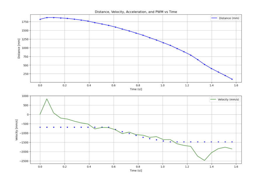
This yielded the following graph that demonstrated high-accuracy for position but moderate deviation at the ends of the velocity estimate through the Kalman Filter (noting that the dots are the previously recorded values and the lines are from the Kalman Filter):

Discussion

This lab was a great chance to integrate the Kalman filter both natively on the robot and through the post-processing software over BLE. It was great to optimize in both Python and C++, providing a greater understanding of computing complex matrices in these coding languages. This lab was completed with Jamison Taylor, and assisted from AI tools for minor debugging.

Summary Lab #7

Configuration

Lab #7 Outcomes

Discussion