Summary Lab #3
Lab #3 is an integration of BLE infrastructure from the previous labs and I2C connection with the ToF sensors. This specifically serves to create an integrated environment for full-scale data collection. Additionally, this includes both design attributes for the sensors and testing optimization with calibration for distance sensing.
Configuration
I2C Sensor Address:
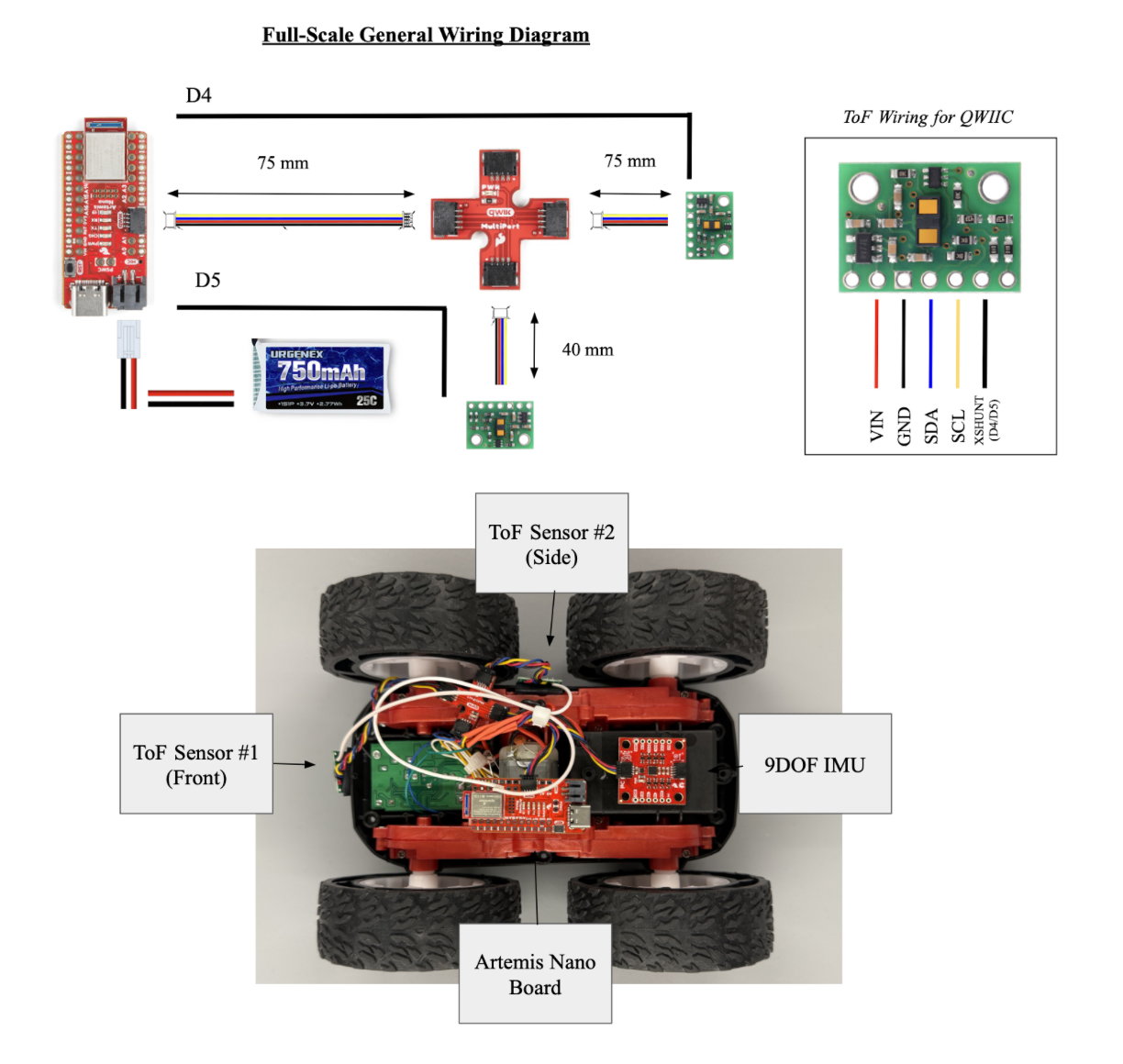
Both Sensors have the same I2C address (0x29) which is expected considering the Polulu VL53L1X ToF sensor has a pre-programmed I2C address set at the factory, specifically 0x29. With the recommended library, these ToF sensors are programmable for I2C addresses between 0x08 and 0x77, with 112 usable addresses. However, this requires connecting to the additional pins on the ToF Sensor boards (XSHUNT and GPIO pins) and running the “sensor.setAddress().” After returning from later sections, I connected XSHUNT for ToF #1 to D4 and ToF #2 to D5 in order to distinguish these two sensors for future usage.
- I2C Sensor #1: 0x29 (Later configured to 0x30)
- I2C Sensor #2: 0x29 (Later configured to 0x31)
2 ToF Sensor Rationale
Two ToF sensors are implemented for distance sensing in order to provide an approximation for objects on a 2D plane. Since the stunt car only maneuvers on a flat plane, objects will only interfere beside or in front of the device (x-axis or y-axis from the car’s frame of reference). With this in mind, one ToF sensor is fixed on the front of the car and another on the lateral side of the car to determine objects relative distance for collision sensing. This system still has flaws, specifically in regards to the precision and full-scale dynamicness of the distance sensing. First, the ToF sensor’s field of view is significantly obstructed by the wheels on the lateral face of the car, causing limited detection for objects diagonal to the stunt car. Second, these sensors only provide detection for 2 of 4 faces of the car, meaning collision detection requires additional configuration to be effective for motions (forward, backwards, tank turns, etc.)
Short, Medium, and Long Range Assessment
hese various modes are efficient depending on the use case of the stunt car. For smaller obstacle courses with tighter turns (i.e. maneuvering within furniture, small mazes, etc.) the short range option is best. For normal-sized rooms with typical spaced obstacles (i.e. door-frames, chairs, etc.), the medium range configuration provides the best dynamic range. For large spaces with few minor obstacles (i.e. clear stadiums, limited objects, etc.), the long range option is the most efficient. For our usage, considering the stunt car will operate primarily inside labs and classrooms, the medium range option is the best and requires the Polulu VL53L1X Library.
Lab #3 Outcomes
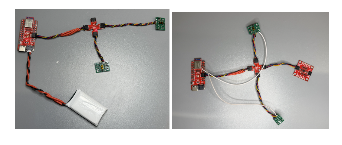
ToF Sensors Connected to QWIIC Breakout Board (With and Without Shunts)
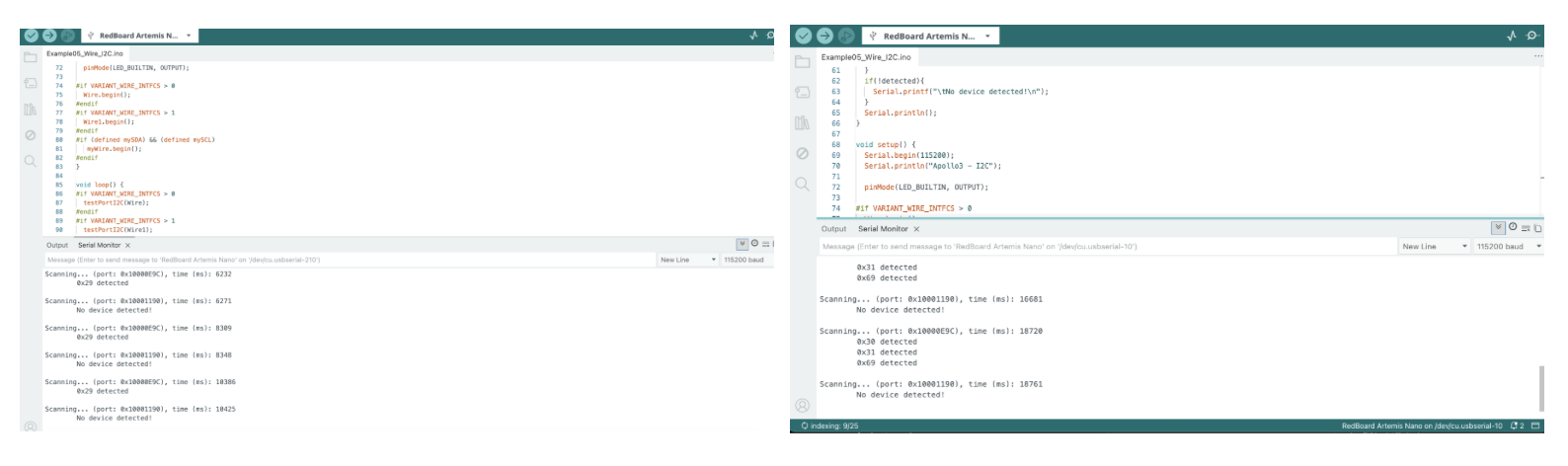
Artemis Scanning for I2C Devices (One ToF, Two ToF and One IMU)
Sensor Data Calibration at Different Levels
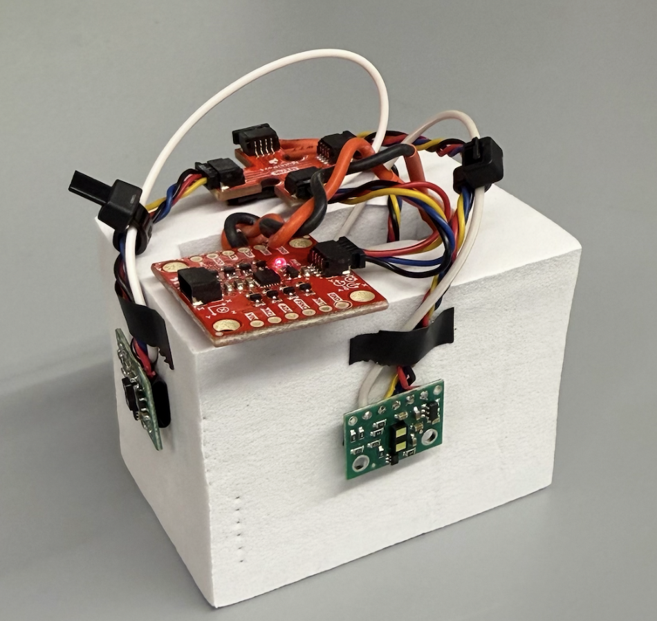
The accuracy and reliability of the Polulu ToF Sensors should be compared across various in-range distances between the two sensors. In order to complete this section of the lab, the 2 ToF sensors, 1 IMU, Artemis Nano Board, and Battery are all assembled onto a makeshift frame in order to complete testing. Here is a clear diagram of the assembled device used for all future testing in the lab:
For this specific case, a calibration curve is developed specifically for the medium-range use case, where 10 discrete measurements are collected comparing the measured distance with the ToF sensor to the actual over a 5 second span, and 2 measurements outside the recommended range. The procedure is written for comparing the accuracy of the other methods given the same experimental set-up:
Procedures
- Short-Scale (0 - 1.3 m): Discrete steps of 0.13 m from the wall between the range of 0.13 m - 1.56 m for both ToF #1 and ToF #2
- Medium-Scale (0 - 3.0 m): Discrete steps of 0.3 m from the wall between the range of 0.3 m - 3.6 m for both ToF #1 and ToF #2
- Long-Scale (0 - 4.0 m): Discrete steps of 0.4 m from the wall between the range of 0.4 m - 4.8 m for both ToF #1 and ToF #2
Relevant Calibration (Medium-Scale)
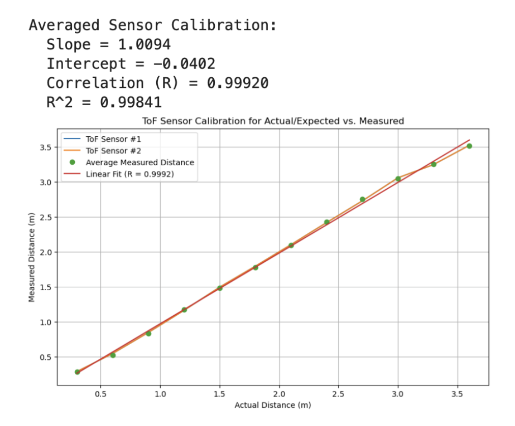
Overall, the sensors demonstrate pretty strong reliability and high-accuracy. By assessing the R^2 value from the average calculated ToF measurement at each location, the higher correlation factor proves consistency among the results during testing. Additionally, with the slope of the line at ~1.01, this is indicative of a highly accurate measurement from the sensors in general. Given the range or accuracy from 0.3 - 3.5 m, this is an additional proof that the medium-range option proves the most dynamic in this circumstance.
import numpy as np

actual = np.array([0.3, 0.6, 0.9, 1.2, 1.5, 1.8, 2.1, 2.4, 2.7, 3.0, 3.3, 3.6])
measured1 = np.array([0.287, 0.544, 0.844, 1.160, 1.492, 1.791, 2.099, 2.415, 2.724, 3.054, 3.244, 3.518])
measured2 = np.array([0.281, 0.508, 0.811, 1.177, 1.465, 1.763, 2.089, 2.441, 2.774, 3.028, 3.255, 3.510])

measured_avg = (measured1 + measured2) / 2

# Linear regression
m_avg, b_avg = np.polyfit(actual, measured_avg, 1)

# Correlation coefficient
r_avg = np.corrcoef(actual, measured_avg)[0, 1]

print("Averaged Sensor Calibration:")
print(f"  Slope = {m_avg:.4f}")
print(f"  Intercept = {b_avg:.4f}")
print(f"  Correlation (R) = {r_avg:.5f}")
print(f"  R^2 = {r_avg**2:.5f}")

import matplotlib.pyplot as plt

fit_avg = m_avg * actual + b_avg

plt.figure(figsize=(10,6))
plt.plot(actual, measured1, label="ToF Sensor #1")
plt.plot(actual, measured1, label="ToF Sensor #2")
plt.plot(actual, measured_avg, 'o', label='Average Measured Distance')
plt.plot(actual, fit_avg, '-', label=f'Linear Fit (R = {r_avg:.4f})')

plt.xlabel("Actual Distance (m)")
plt.ylabel("Measured Distance (m)")
plt.title("ToF Sensor Calibration for Actual/Expected vs. Measured")
plt.legend()
plt.grid(True)
plt.show()
ToF Sensor Speed Optimization
With the Artemis infrastructure, the data streaming within the code could be controlled with greater accuracy during printing in the Serial Monitor. The following is a snippet of the code and screenshots of the ArduinoIDE with this change:
 // -------- DIRECT WIRE MODE --------
 else {
   unsigned long now = millis();
   loop_count++;
   if (myICM.dataReady()) {
     myICM.getAGMT();
   }
   unblockedDistanceToF();
   Serial.print("t(ms): ");
   Serial.print(now);
   Serial.print("ToF #1 (mm): ");
   Serial.print(T1_mm);
   Serial.print("ToF #2 (mm): ");
   Serial.println(T2_mm);
   if (now - last_loop_report >= 1000) {
     Serial.print("Loop Hz: ");
     Serial.println(loop_count);
     loop_count = 0;
     last_loop_report = now;
   }
 }
…
void unblockedDistanceToF(){
 if (ToF_sensor_1.checkForDataReady()) {
   T1_mm = ToF_sensor_1.read(false); // false = do NOT block
   ToF_sensor_1.clearInterrupt();
 }
 if (ToF_sensor_2.checkForDataReady()) {
   T2_mm = ToF_sensor_2.read(false);
   ToF_sensor_2.clearInterrupt();
 }
The major limiting factors within this set-up includes printing to the Serial Monitor and interrupts on the loop, and by integrating the “checkForDataReady” and “clearInterrupt,” the time data streaming is streamlined and controlled.
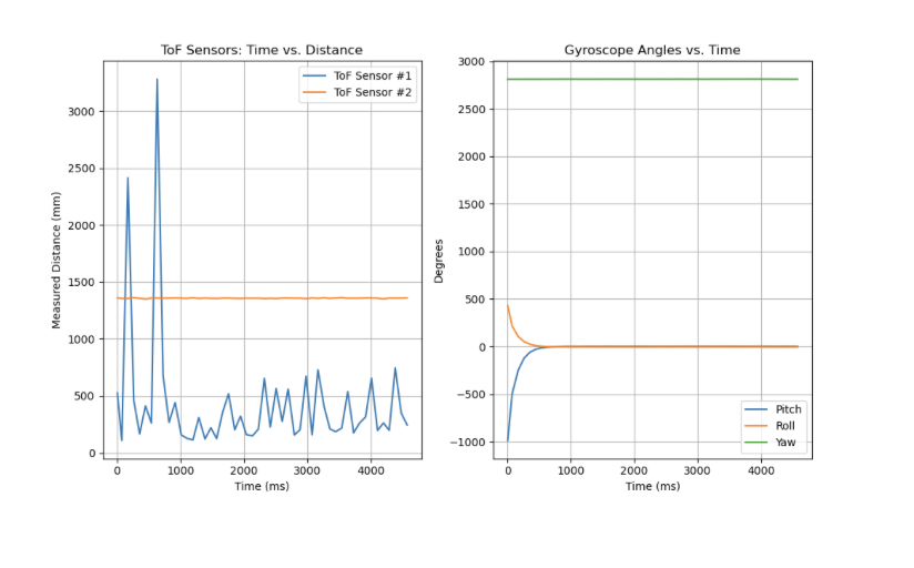
Successful Data Transmission and Graphing with All Sensors
Wireless/ BLE
Wired/ Serial Monitor
Individual Data Transmission from Accelerometer, Gyroscope, and ToF Sensors
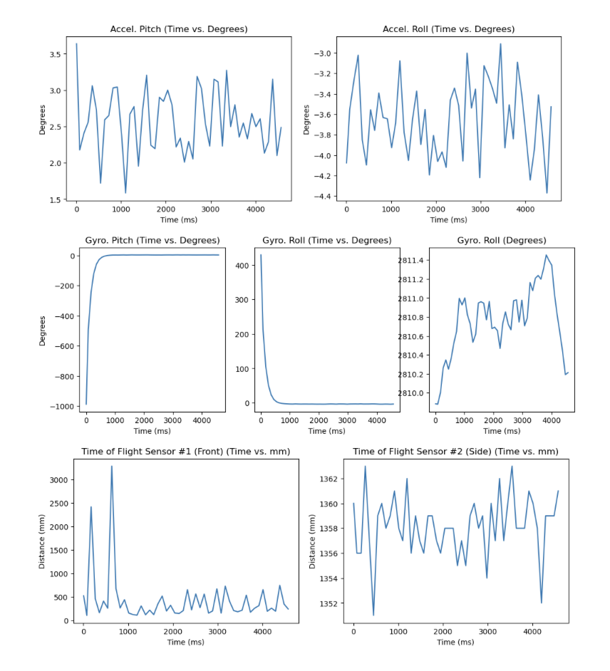
Singular Time vs. Distance from Gyroscope and Time vs. Angle from ToF Sensors
Discussion
This lab was crucial towards integration of learnings from the previous labs and lectures into a usable system for future architecture. With a robust and connected sensor network with both wired and wireless capabilities, I am equipped with the tools to troubleshoot in the future. This lab was completed with Jamison Taylor, with minor AI assistance for code debugging.